Example of generic design in second-level models

This example shows the results obtained in a group analysis using a more complex contrast than a one- or two-sample t test. We use the [left button press (auditory cue)] task from the Localizer dataset and seek association between the contrast values and a variate that measures the speed of pseudo-word reading. No confounding variate is included in the model.

At first, we need to load the Localizer contrasts.

from nilearn.datasets import fetch_localizer_contrasts

n_samples = 94
localizer_dataset = fetch_localizer_contrasts(
    ["left button press (auditory cue)"],
    n_subjects=n_samples,
)

[fetch_localizer_contrasts] Dataset found in /home/remi-gau/nilearn_data/brainomics_localizer

Let’s print basic information on the dataset.

print(
    "First contrast nifti image (3D) is located "
    f"at: {localizer_dataset.cmaps[0]}"
)

First contrast nifti image (3D) is located at: /home/remi-gau/nilearn_data/brainomics_localizer/brainomics_data/S01/cmaps_LeftAuditoryClick.nii.gz

we also need to load the behavioral variable.

tested_var = localizer_dataset.ext_vars["pseudo"]
print(tested_var)

0     15.0
1     16.0
2     14.0
3     19.0
4     16.0
      ...
89    12.0
90    16.0
91    13.0
92    25.0
93    21.0
Name: pseudo, Length: 94, dtype: float64

It is worth to do a quality check and remove subjects with missing values.

import numpy as np

mask_quality_check = np.where(np.logical_not(np.isnan(tested_var)))[0]
n_samples = mask_quality_check.size
contrast_map_filenames = [
    localizer_dataset.cmaps[i] for i in mask_quality_check
]
tested_var = tested_var[mask_quality_check].to_numpy().reshape((-1, 1))
print(f"Actual number of subjects after quality check: {int(n_samples)}")

Actual number of subjects after quality check: 89

Estimate second level model

We define the input maps and the design matrix for the second level model and fit it.

import pandas as pd

design_matrix = pd.DataFrame(
    np.hstack((tested_var, np.ones_like(tested_var))),
    columns=["fluency", "intercept"],
)

Fit of the second-level model

from nilearn.glm.second_level import SecondLevelModel

model = SecondLevelModel(smoothing_fwhm=5.0, n_jobs=2, verbose=1)
model.fit(contrast_map_filenames, design_matrix=design_matrix)

[SecondLevelModel.fit] Fitting second level model. Take a deep breath.
[SecondLevelModel.fit] Loading data from <nibabel.nifti1.Nifti1Image object at 0x7587ebd6ceb0>
[SecondLevelModel.fit] Computing mask
[SecondLevelModel.fit] Resampling mask
[SecondLevelModel.fit] Finished fit
[SecondLevelModel.fit]
Computation of second level model done in 0.30 seconds.

Second Level Model

In a Jupyter environment, please rerun this cell to show the HTML representation or trust the notebook.
On GitHub, the HTML representation is unable to render, please try loading this page with nbviewer.org.

To estimate the contrast is very simple. We can just provide the column name of the design matrix.

z_map = model.compute_contrast("fluency", output_type="z_score")

[SecondLevelModel.compute_contrast] Loading data from <nibabel.nifti1.Nifti1Image object at 0x7587ebd6cf10>
[SecondLevelModel.compute_contrast] Smoothing images
[SecondLevelModel.compute_contrast] Extracting region signals
[SecondLevelModel.compute_contrast] Cleaning extracted signals
[SecondLevelModel.compute_contrast] Computing image from signals

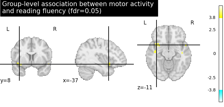
We compute the fdr-corrected p = 0.05 threshold for these data.

from nilearn.glm import threshold_stats_img

_, threshold = threshold_stats_img(z_map, alpha=0.05, height_control="fdr")

Let us plot the second level contrast at the computed thresholds.

from nilearn.plotting import plot_stat_map, show

cut_coords = [10, -5, 10]

plot_stat_map(
    z_map,
    threshold=threshold,
    title="Group-level association between motor activity \n"
    "and reading fluency (fdr=0.05)",
    cut_coords=cut_coords,
    draw_cross=False,
)

show()

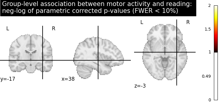
Computing the (corrected) p-values with parametric test to compare with non parametric test

from nilearn.image import get_data, math_img

p_val = model.compute_contrast("fluency", output_type="p_value")
n_voxels = np.sum(get_data(model.masker_.mask_img_))
# Correcting the p-values for multiple testing and taking negative logarithm
neg_log_pval = math_img(
    f"-np.log10(np.minimum(1, img * {n_voxels!s}))", img=p_val
)

[SecondLevelModel.compute_contrast] Loading data from <nibabel.nifti1.Nifti1Image object at 0x7587ebd6d5a0>
[SecondLevelModel.compute_contrast] Smoothing images
[SecondLevelModel.compute_contrast] Extracting region signals
[SecondLevelModel.compute_contrast] Cleaning extracted signals
[SecondLevelModel.compute_contrast] Computing image from signals
<string>:1: RuntimeWarning: divide by zero encountered in log10

Let us plot the (corrected) negative log p-values for the parametric test

# Since we are plotting negative log p-values and using a threshold equal to 1,
# it corresponds to corrected p-values lower than 10%, meaning that there
# is less than 10% probability to make a single false discovery
# (90% chance that we make no false discoveries at all).
# This threshold is much more conservative than the previous one.
threshold = 1
title = (
    "Group-level association between motor activity and reading: \n"
    "neg-log of parametric corrected p-values (FWER < 10%)"
)
plot_stat_map(
    neg_log_pval,
    cut_coords=cut_coords,
    threshold=threshold,
    title=title,
    vmin=threshold,
    cmap="inferno",
    draw_cross=False,
)
show()

/home/remi-gau/github/nilearn/nilearn/examples/05_glm_second_level/plot_second_level_association_test.py:119: UserWarning: Non-finite values detected. These values will be replaced with zeros.
  plot_stat_map(

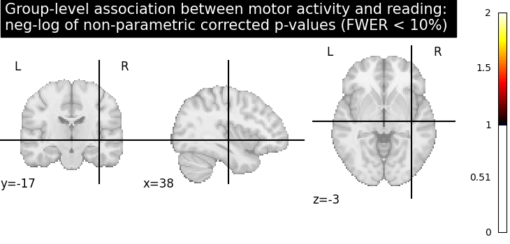
Computing the (corrected) negative log p-values with permutation test

from nilearn.glm.second_level import non_parametric_inference

neg_log_pvals_permuted_ols_unmasked = non_parametric_inference(
    contrast_map_filenames,
    design_matrix=design_matrix,
    second_level_contrast="fluency",
    model_intercept=True,
    n_perm=1000,
    two_sided_test=False,
    mask=None,
    smoothing_fwhm=5.0,
    n_jobs=2,
    verbose=1,
)

[non_parametric_inference] Fitting second level model...
[non_parametric_inference]
Computation of second level model done in 0.2895982265472412 seconds

Let us plot the (corrected) negative log p-values

title = (
    "Group-level association between motor activity and reading: \n"
    "neg-log of non-parametric corrected p-values (FWER < 10%)"
)
plot_stat_map(
    neg_log_pvals_permuted_ols_unmasked,
    cut_coords=cut_coords,
    threshold=threshold,
    title=title,
    vmin=threshold,
    cmap="inferno",
    draw_cross=False,
)
show()

# The neg-log p-values obtained with non parametric testing are capped at 3
# since the number of permutations is 1e3.
# The non parametric test yields a few more discoveries
# and is then more powerful than the usual parametric procedure.

Estimated memory usage: 151 MB