Note
This page is a reference documentation. It only explains the function signature, and not how to use it. Please refer to the user guide for the big picture.
nilearn.plotting.plot_img
- nilearn.plotting.plot_img(img, cut_coords=None, output_file=None, display_mode='ortho', figure=None, axes=None, title=None, threshold=None, annotate=True, draw_cross=True, black_bg=False, colorbar=True, cbar_tick_format='%.2g', resampling_interpolation='continuous', bg_img=None, vmin=None, vmax=None, radiological=False, decimals=False, cmap='gray', transparency=None, transparency_range=None, **kwargs)[source]
Plot cuts of a given image.
By default Frontal, Axial, and Lateral.
- Parameters:
- imgNiimg-like object
- cut_coordsNone, allowed types depend on the
display_mode, optional The world coordinates of the point where the cut is performed.
If
display_modeis'ortho'or'tiled', this must be a 3-sequence offloatorint:(x, y, z).If
display_modeis'xz','yz'or'yx', this must be a 2-sequence offloatorint:(x, z),(y, z)or(x, y).If
display_modeis"x","y", or"z", this can be:If
display_modeis'mosaic', this can be:an
intin which case it specifies the number of cuts to perform in each direction"x","y","z".a 3-sequence of
floatorintin which case it specifies the number of cuts to perform in each direction"x","y","z"separately.dict<str: 1Dndarray> in which case keys are the directions (‘x’, ‘y’, ‘z’) and the values are sequences holding the cut coordinates.
If
Noneis given, the cuts are calculated automatically.
- output_file
strorpathlib.Pathor None, default=None The name of an image file to export the plot to. Valid extensions are .png, .pdf, .svg. If output_file is not None, the plot is saved to a file, and the display is closed.
- display_mode{“ortho”, “tiled”, “mosaic”, “x”, “y”, “z”, “yx”, “xz”, “yz”}, default=”ortho”
Choose the direction of the cuts:
"x": sagittal"y": coronal"z": axial"ortho": three cuts are performed in orthogonal directions"tiled": three cuts are performed and arranged in a 2x2 grid"mosaic": three cuts are performed along multiple rows and columns
- figure
int, ormatplotlib.figure.Figure, or None, optional Matplotlib figure used or its number. If None is given, a new figure is created.
- axes
matplotlib.axes.Axes, or 4tupleoffloat: (xmin, ymin, width, height), default=None The axes, or the coordinates, in matplotlib figure space, of the axes used to display the plot. If None, the complete figure is used.
- title
str, or None, default=None The title displayed on the figure.
- threshold
intorfloat,str, None, or ‘auto’, optional If None is given, the image is not thresholded. If number is given, it must be non-negative. The specified value is used to threshold the image: values below the threshold (in absolute value) are plotted as transparent. If a string percentile is given, it should finish with percent sign e.g., “95%”. We threshold based on the score obtained using this percentile on the image data. If “auto” is given, the threshold is determined based on the score obtained using percentile value “80%” on the absolute value of the image data.
- annotate
bool, default=True If annotate is True (like positions and / or left/right annotation) are added to the plot.
- draw_cross
bool, default=True If draw_cross is True, a cross is drawn on the plot to indicate the cut position.
- black_bg
bool, or “auto”, optional If True, the background of the image is set to be black. If you wish to save figures with a black background, you will need to pass facecolor=”k”, edgecolor=”k” to
matplotlib.pyplot.savefig. default=False.- colorbar
bool, optional If True, display a colorbar next to the plots. default=True.
- cbar_tick_format
str, default=”%.2g” (scientific notation) Controls how to format the tick labels of the colorbar. Ex: use “%i” to display as integers.
- resampling_interpolation
str, optional Interpolation to use when resampling the image to the destination space. Can be:
"continuous": use 3rd-order spline interpolation"nearest": use nearest-neighbor mapping.
Note
"nearest"is faster but can be noisier in some cases.default=’continuous’.
- bg_imgNiimg-like object, optional
See Input and output: neuroimaging data representation. The background image to plot on top of. If nothing is specified, no background image is plotted. default=None.
- vmin
floator obj:int or None, optional Lower bound of the colormap. The values below vmin are masked. If None, the min of the image is used. Passed to
matplotlib.pyplot.imshow.- vmax
floator obj:int or None, optional Upper bound of the colormap. The values above vmax are masked. If None, the max of the image is used. Passed to
matplotlib.pyplot.imshow.- radiological
bool, default=False Invert x axis and R L labels to plot sections as a radiological view. If False (default), the left hemisphere is on the left of a coronal image. If True, left hemisphere is on the right.
- decimals
intorbool, default=False Number of decimal places on slice position annotation. If False, the slice position is integer without decimal point.
- cmap
matplotlib.colors.Colormap, orstr, optional The colormap to use. Either a string which is a name of a matplotlib colormap, or a matplotlib colormap object. default=”gray”
- transparency
floatbetween 0 and 1, or a Niimg-Like object, or None, default = None Value to be passed as alpha value to
imshow. ifNoneis passed, it will be set to 1. If an image is passed, voxel-wise alpha blending will be applied, by relying on the absolute value oftransparencyat each voxel.Added in Nilearn 0.12.0.
- transparency_range
tupleorlistof 2 non-negative numbers, or None, default = None When an image is passed to
transparency, this determines the range of values in the image to use for transparency (alpha blending). For example withtransparency_range = [1.96, 3], any voxel / vertex ( ):
):with a value between between -1.96 and 1.96, would be fully transparent (alpha = 0),
with a value less than -3 or greater than 3, would be fully opaque (alpha = 1),
with a value in the intervals
[-3.0, -1.96]or[1.96, 3.0], would have an alpha_i value scaled linearly between 0 and 1 : .
.
This parameter will be ignored unless an image is passed as
transparency. The first number must be greater than 0 and less than the second one. ifNoneis passed, this will be set to[0, max(abs(transparency))].Added in Nilearn 0.12.0.
- kwargsextra keyword arguments, optional
Extra keyword arguments ultimately passed to matplotlib.pyplot.imshow via
add_overlay.
- Returns:
- display
OrthoSliceror None An instance of the OrthoSlicer class. If
output_fileis defined, None is returned.
- display
- Raises:
- ValueError
if the specified threshold is a negative number
See also
plot_anatTo simply plot anatomical images
plot_epiTo simply plot raw EPI images
plot_roiTo simply plot max-prob atlases (3D images)
plot_prob_atlasTo simply plot probabilistic atlases (4D images)
nilearn.plottingSee API reference for other options
Notes
This is a low-level function. For most use cases, other plotting functions might be more appropriate and easier to use.
Examples
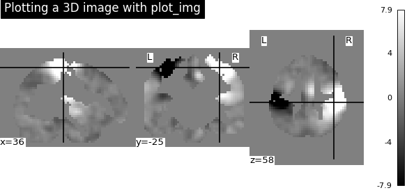
>>> from nilearn.plotting.image.img_plotting import plot_img, show
>>> from nilearn.datasets import load_sample_motor_activation_image
>>>
>>> # just to have a 3D image with some structure
>>> data = load_sample_motor_activation_image()
>>>
>>> display = plot_img(data, title="Plotting a 3D image with plot_img")
>>> show()
Examples using nilearn.plotting.plot_img
Basic nilearn example: manipulating and looking at data
Intro to GLM Analysis: a single-run, single-subject fMRI dataset