5.5. Searchlight : finding voxels containing information

This page overviews searchlight analyses and how they are approached in nilearn with the SearchLight estimator.

5.5.1. Principle of the Searchlight

SearchLight analysis was introduced in [Kriegeskorte et al.[3]], and consists of scanning the brain with a searchlight. Briefly, a ball of given radius is scanned across the brain volume and the prediction accuracy of a classifier trained on the corresponding voxels is measured.

Searchlights are also not limited to classification; regression (e.g., [Kahnt et al.[4]]) and representational similarity analysis (e.g., [Clarke and Tyler[5]]) are other uses of searchlights. Currently, only classification and regression are supported in nilearn.

Further Reading

For a critical review on searchlights, see [Etzel et al.[6]].

5.5.2. Preparing the data

SearchLight requires a series of brain volumes as input, X, each with a corresponding label, y. The number of brain volumes therefore correspond to the number of samples used for decoding.

5.5.2.1. Masking

One of the main elements that distinguish SearchLight from other algorithms is the notion of structuring element that scans the entire volume. This has an impact on the masking procedure.

Two masks are used with SearchLight:

• mask_img is the anatomical mask

• process_mask_img is a subset of the brain mask and defines the boundaries of where the searchlight scans the volume. Often times we are interested in only performing a searchlight within a specific area of the brain (e.g., frontal cortex). If no process_mask_img is set, then nilearn.decoding.SearchLight defaults to performing a searchlight over the whole brain.

mask_img ensures that only voxels with usable signals are included in the searchlight. This could be a full-brain mask or a gray-matter mask.

5.5.3. Setting up the searchlight

5.5.3.1. Classifier

The classifier used by default by SearchLight is LinearSVC with C=1 but this can be customized easily by passing an estimator parameter to the Searchlight. See scikit-learn documentation for other classifiers. You can also pass scikit-learn Pipelines to the SearchLight in order to combine estimators and preprocessing steps (e.g., feature scaling) for your searchlight.

5.5.3.2. Score function

Metrics can be specified by the “scoring” argument to the SearchLight, as detailed in the scikit-learn documentation

5.5.3.3. Cross validation

SearchLight will iterate on the volume and give a score to each voxel. This score is computed by running a classifier on selected voxels. In order to make this score as accurate as possible (and avoid overfitting), cross-validation is used.

Cross-validation can be defined using the “cv” argument. As it is computationally costly, K-Fold cross validation with K = 3 is set as the default. A scikit-learn cross-validation generator can also be passed to set a specific type of cross-validation.

Leave-one-run-out cross-validation (LOROCV) is a common approach for searchlights. This approach is a specific use-case of grouped cross-validation, where the cross-validation folds are determined by the acquisition runs. The held-out fold in a given iteration of cross-validation consist of data from a separate run, which keeps training and validation sets properly independent. For this reason, LOROCV is often recommended. This can be performed by using LeaveOneGroupOut, and then setting the group/run labels when fitting the estimator.

5.5.3.4. Sphere radius

An important parameter is the radius of the sphere that will run through the data. The sphere size determines the number of voxels/features to use for classification (i.e. more voxels are included with larger spheres).

Note

SearchLight defines sphere radius in millimeters; the number of voxels included in the sphere will therefore depend on the voxel size.

For reference, [Kriegeskorte et al.[3]] use a 4mm radius because it yielded the best detection performance in their simulation of 2mm isovoxel data.

5.5.4. Visualization

5.5.4.1. Searchlight

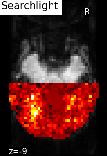
The results of the searchlight can be found in the scores_ attribute of the SearchLight object after fitting it to the data. Below is a visualization of the results from Searchlight analysis of face vs house recognition. The searchlight was restricted to a slice in the back of the brain. Within this slice, we can see that a cluster of voxels in visual cortex contains information to distinguish pictures showed to the volunteers, which was the expected result.

See also

• Plotting brain images

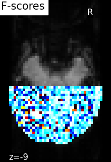
5.5.4.2. Comparing to massively univariate analysis: F_score or SPM

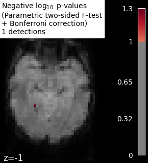
The standard approach to brain mapping is performed using Statistical Parametric Mapping (SPM), using ANOVA (analysis of variance), and parametric tests (F-tests ot t-tests). Here we compute the p-values of the voxels [1]. To display the results, we use the negative log of the p-value.

Parametric scores can be converted into p-values using a reference theoretical distribution, which is known under specific assumptions (hence the name parametric). In practice, neuroimaging signal has a complex structure that might not match these assumptions. An exact, non-parametric permutation test can be performed as an alternative to the parametric test: the residuals of the model are permuted so as to break any effect and the corresponding decision statistic is recomputed. One thus builds the distribution of the decision statistic under the hypothesis that there is no relationship between the tested variates and the target variates. In neuroimaging, this is generally done by swapping the signal values of all voxels while the tested variables remain unchanged [2]. A voxel-wise analysis is then performed on the permuted data. The relationships between the image descriptors and the tested variates are broken while the value of the signal in each particular voxel can be observed with the same probability than the original value associated to that voxel. Note that it is hereby assumed that the signal distribution is the same in every voxel. Several data permutations are performed (typically 10,000) while the scores for every voxel and every data permutation is stored. The empirical distribution of the scores is thus constructed (under the hypothesis that there is no relationship between the tested variates and the neuroimaging signal, the so-called null-hypothesis) and we can compare the original scores to that distribution: The higher the rank of the original score, the smaller is its associated p-value. The nilearn.mass_univariate.permuted_ols function returns the p-values computed with a permutation test.

The number of tests performed is generally large when full-brain analysis is performed (> 50,000 voxels). This increases the probability of finding a significant activation by chance, a phenomenon that is known to statisticians as the multiple comparisons problem. It is therefore recommended to correct the p-values to take into account the multiple tests. Bonferroni correction consists of multiplying the p-values by the number of tests (while making sure the p-values remain smaller than 1). Thus, we control the occurrence of one false detection at most, the so-called family-wise error control. A similar control can be performed when performing a permutation test: For each permutation, only the maximum value of the F-statistic across voxels is considered and is used to build the null distribution. It is crucial to assume that the distribution of the signal is the same in every voxel so that the F-statistics are comparable. This correction strategy is applied in nilearn nilearn.mass_univariate.permuted_ols function.

We observe that the results obtained with a permutation test are less conservative than the ones obtained with a Bonferroni correction strategy.

In nilearn nilearn.mass_univariate.permuted_ols function, we permute a parametric t-test. Unlike F-test, a t-test can be signed (one-sided test), that is both the absolute value and the sign of an effect are considered. Thus, only positive effects can be focused on. It is still possible to perform a two-sided test equivalent to a permuted F-test by setting the argument two_sided_test to True. In the example above, we do perform a two-sided test but add back the sign of the effect at the end using the t-scores obtained on the original (non-permuted) data. Thus, we can perform two one-sided tests (a given contrast and its opposite) for the price of one single run. The example results can be interpreted as follows: viewing faces significantly activates the Fusiform Face Area as compared to viewing houses, while viewing houses does not reveal significant supplementary activations as compared to viewing faces.

[1]

The p-value is the probability of getting the observed values assuming that nothing happens (i.e. under the null hypothesis). Therefore, a small p-value indicates that there is a small chance of getting this data if no real difference existed, so the observed voxel must be significant.

[2]

When the variate tested is a scalar (test of the intercept) –which corresponds to a one sample test–, no swapping can be performed but one can estimate the null distribution by assuming symmetry about some reference value. When this value is zero, one can randomly swap the sign of the target variates (the imaging signal). nilearn nilearn.mass_univariate.permuted_ols function automatically adopts the suitable strategy according to the input data.

Example code

All the steps discussed in this section can be seen implemented in a full code example.

5.5.5. References

[3] (1,2)

Nikolaus Kriegeskorte, Rainer Goebel, and Peter Bandettini. Information-based functional brain mapping. Proceedings of the National Academy of Sciences, 103(10):3863–3868, 2006. URL: https://www.pnas.org/content/103/10/3863, doi:10.1073/pnas.0600244103.

[4]

Thorsten Kahnt, Marcus Grueschow, Oliver Speck, and John-Dylan Haynes. Perceptual learning and decision-making in human medial frontal cortex. Neuron, 70(3):549–559, 2011. URL: https://www.sciencedirect.com/science/article/pii/S0896627311002960, doi:https://doi.org/10.1016/j.neuron.2011.02.054.

[5]

Alex Clarke and Lorraine K. Tyler. Object-specific semantic coding in human perirhinal cortex. Journal of Neuroscience, 34(14):4766–4775, 2014. URL: https://www.jneurosci.org/content/34/14/4766, arXiv:https://www.jneurosci.org/content/34/14/4766.full.pdf, doi:10.1523/JNEUROSCI.2828-13.2014.

[6]

Joset A. Etzel, Jeffrey M. Zacks, and Todd S. Braver. Searchlight analysis: promise, pitfalls, and potential. NeuroImage, 78:261–269, 2013. URL: https://www.sciencedirect.com/science/article/pii/S1053811913002917, doi:https://doi.org/10.1016/j.neuroimage.2013.03.041.