6.4. Region Extraction for better brain parcellations#

6.4.1. Fetching movie-watching based functional datasets#

We use a naturalistic stimuli based movie-watching functional connectivity dataset of 20 subjects, which is already preprocessed, downsampled to 4mm isotropic resolution, and publicly available at https://osf.io/5hju4/files/. We use utilities fetch_development_fmri implemented in nilearn for automatic fetching of this dataset.

from nilearn import datasets

rest_dataset = datasets.fetch_development_fmri(n_subjects=20)
func_filenames = rest_dataset.func
confounds = rest_dataset.confounds

6.4.2. Brain maps using Dictionary learning #

Here, we use object DictLearning, a multi subject model to decompose multi subjects fMRI datasets into functionally defined maps. We do this by setting the parameters and calling DictLearning.fit on the filenames of datasets without necessarily converting each file to Nifti1Image object.

from nilearn.decomposition import DictLearning

# Initialize DictLearning object
dict_learn = DictLearning(
    n_components=8,
    smoothing_fwhm=6.0,
    memory="nilearn_cache",
    memory_level=2,
    random_state=0,
    standardize="zscore_sample",
)
# Fit to the data
dict_learn.fit(func_filenames)
# Resting state networks/maps in attribute `components_img_`
components_img = dict_learn.components_img_

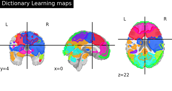
6.4.3. Visualization of Dictionary learning maps#

Showing maps stored in components_img using nilearn plotting utilities. Here, we use plot_prob_atlas for easy visualization of 4D atlas maps onto the anatomical standard template. Each map is displayed in different color and colors are random and automatically picked.

from nilearn import plotting

plotting.plot_prob_atlas(
    components_img,
    view_type="filled_contours",
    title="Dictionary Learning maps",
)

6.4.4. Region Extraction with Dictionary learning maps#

We use object RegionExtractor for extracting brain connected regions from dictionary maps into separated brain activation regions with automatic thresholding strategy selected as thresholding_strategy='ratio_n_voxels'. We use thresholding strategy to first get foreground information present in the maps and then followed by robust region extraction on foreground information using Random Walker algorithm selected as extractor='local_regions'.

Here, we control foreground extraction using parameter threshold=.5, which represents the expected proportion of voxels included in the regions (i.e. with a non-zero value in one of the maps). If you need to keep more proportion of voxels then threshold should be tweaked according to the maps data.

The parameter min_region_size=1350 mm^3 is to keep the minimum number of extracted regions. We control the small spurious regions size by thresholding in voxel units to adapt well to the resolution of the image. Please see the documentation of connected_regions for more details.

from nilearn.regions import RegionExtractor

extractor = RegionExtractor(
    components_img,
    threshold=0.5,
    thresholding_strategy="ratio_n_voxels",
    extractor="local_regions",
    standardize="zscore_sample",
    standardize_confounds="zscore_sample",
    min_region_size=1350,
)
# Just call fit() to process for regions extraction
extractor.fit()
# Extracted regions are stored in regions_img_
regions_extracted_img = extractor.regions_img_
# Each region index is stored in index_
regions_index = extractor.index_
# Total number of regions extracted
n_regions_extracted = regions_extracted_img.shape[-1]

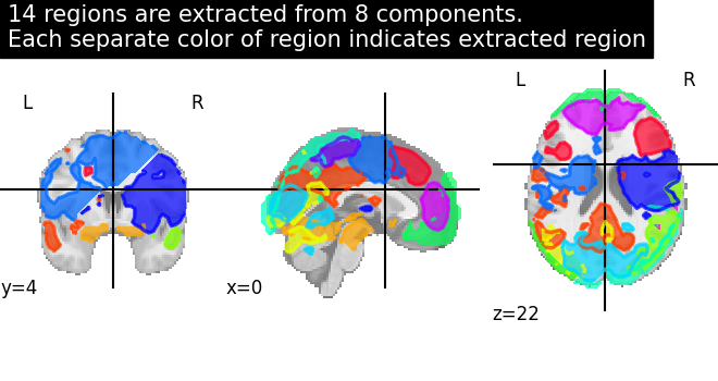
6.4.5. Visualization of Region Extraction results#

Showing region extraction results. The same function plot_prob_atlas is used for visualizing extracted regions on a standard template. Each extracted brain region is assigned a color and as you can see that visual cortex area is extracted quite nicely into each hemisphere.

title = (
    "%d regions are extracted from %d components."
    "\nEach separate color of region indicates extracted region"
    % (n_regions_extracted, 8)
)
plotting.plot_prob_atlas(
    regions_extracted_img, view_type="filled_contours", title=title
)

6.4.6. Computing functional connectivity matrices#

Here, we use the object called ConnectivityMeasure to compute functional connectivity measured between each extracted brain regions. Many different kinds of measures exists in nilearn such as “correlation”, “partial correlation”, “tangent”, “covariance”, “precision”. But, here we show how to compute only correlations by selecting parameter as kind='correlation' as initialized in the object.

The first step to do is to extract subject specific time series signals using functional data stored in func_filenames and the second step is to call ConnectivityMeasure.fit_transform on the time series signals. Here, for each subject we have time series signals of shape=(168, n_regions_extracted) where 168 is the length of time series and n_regions_extracted is the number of extracted regions. Likewise, we have a total of 20 subject specific time series signals. The third step, we compute the mean correlation across all subjects.

from nilearn.connectome import ConnectivityMeasure

correlations = []
# Initializing ConnectivityMeasure object with kind='correlation'
connectome_measure = ConnectivityMeasure(
    kind="correlation",
    standardize="zscore_sample",
)
for filename, confound in zip(func_filenames, confounds):
    # call transform from RegionExtractor object to extract timeseries signals
    timeseries_each_subject = extractor.transform(filename, confounds=confound)
    # call fit_transform from ConnectivityMeasure object
    correlation = connectome_measure.fit_transform([timeseries_each_subject])
    # saving each subject correlation to correlations
    correlations.append(correlation)

# Mean of all correlations
import numpy as np

mean_correlations = np.mean(correlations, axis=0).reshape(
    n_regions_extracted, n_regions_extracted
)

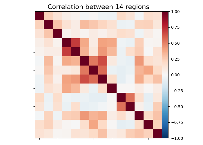
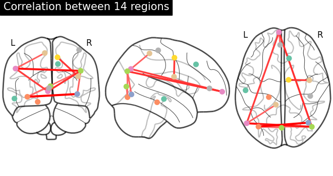
6.4.7. Visualization of functional connectivity matrices#

Showing mean of correlation matrices computed between each extracted brain regions. At this point, we make use of nilearn image and plotting utilities to find automatically the coordinates required, for plotting connectome relations. Left image is the correlations in a matrix form and right image is the connectivity relations to brain regions plotted using plot_connectome

title = f"Correlation between {int(n_regions_extracted)} regions"

# First plot the matrix
display = plotting.plot_matrix(
    mean_correlations, vmax=1, vmin=-1, colorbar=True, title=title
)

# Then find the center of the regions and plot a connectome
regions_img = regions_extracted_img
coords_connectome = plotting.find_probabilistic_atlas_cut_coords(regions_img)

plotting.plot_connectome(
    mean_correlations, coords_connectome, edge_threshold="90%", title=title
)

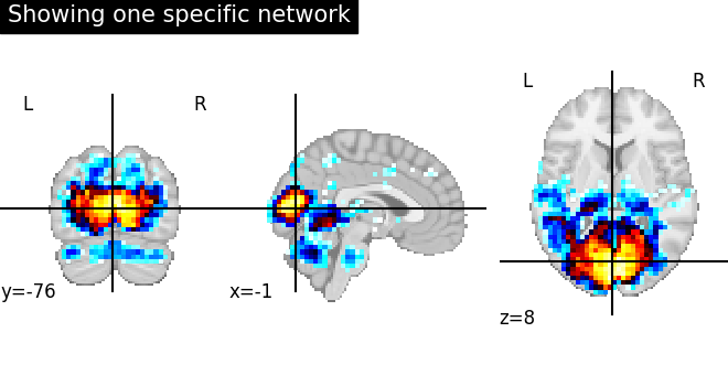
6.4.8. Validating results#

Showing only one specific network regions before and after region extraction. The first image displays the regions of one specific functional network without region extraction.

from nilearn import image

img = image.index_img(components_img, 4)
coords = plotting.find_xyz_cut_coords(img)
display = plotting.plot_stat_map(
    img,
    cut_coords=coords,
    colorbar=False,
    title="Showing one specific network",
)

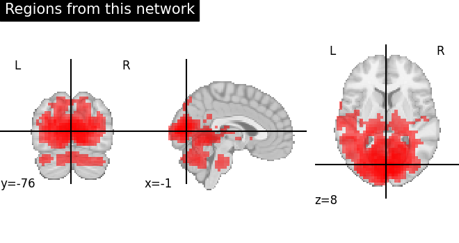
The second image displays the regions split apart after region extraction. Here, we can validate that regions are nicely separated identified by each extracted region in different color.

regions_indices_of_map3 = np.where(np.array(regions_index) == 4)

display = plotting.plot_anat(
    cut_coords=coords, title="Regions from this network"
)

# Add as an overlay all the regions of index 4
colors = "rgbcmyk"
for each_index_of_map3, color in zip(regions_indices_of_map3[0], colors):
    display.add_overlay(
        image.index_img(regions_extracted_img, each_index_of_map3),
        cmap=plotting.cm.alpha_cmap(color),
    )

plotting.show()

# sphinx_gallery_dummy_images=6