9.3. From neuroimaging volumes to data matrices: the masker objects

This chapter introduces the maskers: objects that go from neuroimaging volumes, on the disk or in memory, to data matrices, eg of time series.

9.3.1. The concept of “masker” objects

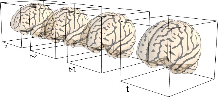
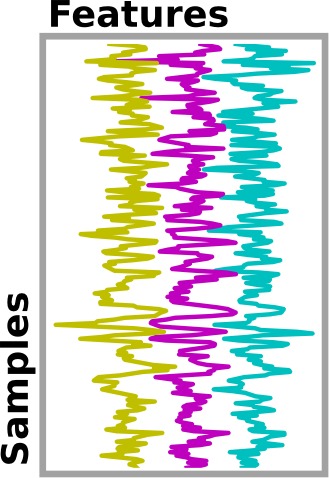
In any analysis, the first step is to load the data. It is often convenient to apply some basic data transformations and to turn the data in a 2D (samples x features) matrix, where the samples could be different time points, and the features derived from different voxels (e.g., restrict analysis to the ventral visual stream), regions of interest (e.g., extract local signals from spheres/cubes), or pre-specified networks (e.g., look at data from all voxels of a set of network nodes). Think of masker objects as swiss-army knives for shaping the raw neuroimaging data in 3D space into the units of observation relevant for the research questions at hand.

Tip

Masker objects can transform both 3D and 4D image objects. Transforming a 4D image produces a 2D (samples x features) matrix. Currently, transforming a 3D image also produces a 2D (1 x features) matrix, but starting in version 0.12, it will produce a 1D (features) array.

→

“masker” objects (found in module nilearn.maskers) simplify these “data folding” steps that often precede the statistical analysis.

Note that the masker objects may not cover all the image transformations for specific tasks. Users who want to make some specific processing may have to call specific functions (modules nilearn.signal, nilearn.masking).

Advanced: Design philosophy of “Maskers”

The design of these classes is similar to scikit-learn‘s transformers. First, objects are initialized with some parameters guiding the transformation (unrelated to the data). Then the fit() method should be called, possibly specifying some data-related information (such as number of images to process), to perform some initial computation (e.g., fitting a mask based on the data). Finally, transform() can be called, with the data as argument, to perform some computation on data themselves (e.g., extracting time series from images).

9.3.2. NiftiMasker: applying a mask to load time-series

NiftiMasker is a powerful tool to load images and extract voxel signals in the area defined by the mask. It applies some basic preprocessing steps with commonly used parameters as defaults. But it is very important to look at your data to see the effects of the preprocessings and validate them.

Advanced: scikit-learn Pipelines

NiftiMasker is a scikit-learn compliant transformer so that you can directly plug it into a scikit-learn pipeline.

9.3.2.1. Custom data loading: loading only the first 100 time points

Suppose we want to restrict a dataset to the first 100 frames. Below, we load a movie-watching dataset with fetch_development_fmri(), restrict it to 100 frames and build a new niimg object that we can give to the masker. Although possible, there is no need to save your data to a file to pass it to a NiftiMasker. Simply use nilearn.image.index_img to apply a slice and create a Niimg in memory:

dataset = datasets.fetch_development_fmri(n_subjects=1)
epi_filename = dataset.func[0]

# Restrict to 100 frames to speed up computation
from nilearn.image import index_img

epi_img = index_img(epi_filename, slice(0, 100))

9.3.2.2. Controlling how the mask is computed from the data

In this section, we show how the masker object can compute a mask automatically for subsequent statistical analysis. On some datasets, the default algorithm may however perform poorly. This is why it is very important to always look at your data before and after feature engineering using masker objects.

Note

The full example described in this section can be found here: plot_mask_computation.py. It is also related to this example: plot_nifti_simple.py.

9.3.2.2.1. Visualizing the computed mask

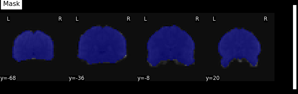
If a mask is not specified as an argument, NiftiMasker will try to compute one from the provided neuroimaging data. It is very important to verify the quality of the generated mask by visualization. This allows to see whether it is suitable for your data and intended analyses. Alternatively, the mask computation parameters can still be modified. See the NiftiMasker documentation for a complete list of mask computation parameters.

The mask can be retrieved and visualized from the mask_img_ attribute of the masker:

masker = NiftiMasker()
masker.fit(miyawaki_filename)

# Plot the generated mask using the mask_img_ attribute
plot_roi(
    masker.mask_img_, miyawaki_mean_img, title="Mask from already masked data"
)

# %%

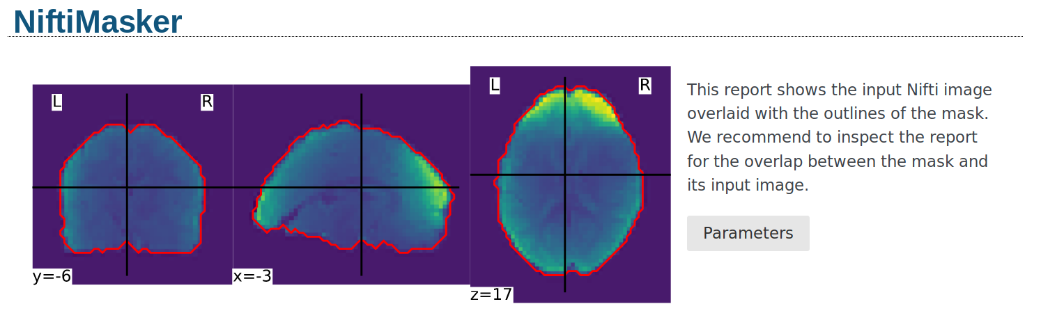
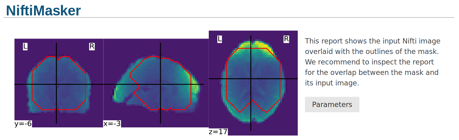
Alternatively, the mask can be visualized using the generate_report method of the masker. The generated report can be viewed in a Jupyter notebook, opened in a new browser tab using report.open_in_browser(), or saved as a portable HTML file report.save_as_html(output_filepath).

masker = NiftiMasker(mask_strategy="epi")
masker.fit(epi_img)
report = masker.generate_report()
report

# %%

9.3.2.2.2. Different masking strategies

The mask_strategy argument controls how the mask is computed:

• background: detects a continuous background

• epi: suitable for EPI images

• whole-brain-template: uses an MNI whole-brain template

• gm-template: uses an MNI grey-matter template

• wm-template: uses an MNI white-matter template

9.3.2.2.3. Extra mask parameters: opening, cutoff…

The underlying function is nilearn.masking.compute_epi_mask called using the mask_args argument of the NiftiMasker. Controlling these arguments set the fine aspects of the mask. See the functions documentation, or the NiftiMasker example.

9.3.2.3. Common data preparation steps: smoothing, filtering, resampling

NiftiMasker comes with many parameters that enable data preparation:

>>> import sklearn; sklearn.set_config(print_changed_only=False)
>>> from nilearn import maskers
>>> masker = maskers.NiftiMasker()
>>> masker 
NiftiMasker(detrend=False, dtype=None, high_pass=None,
      high_variance_confounds=False, low_pass=None, mask_args=None,
      mask_img=None, mask_strategy='background',
      memory=Memory(location=None), memory_level=1, reports=True,
      runs=None, smoothing_fwhm=None, standardize=False,
      standardize_confounds=True, t_r=None,
      target_affine=None, target_shape=None, verbose=0)

The meaning of each parameter is described in the documentation of NiftiMasker (click on the name NiftiMasker), here we comment on the most important.

`dtype` argument

Forcing your data to have a dtype of float32 can help save memory and is often a good-enough numerical precision. You can force this cast by choosing dtype to be ‘auto’. In the future this cast will be the default behaviour.

See also

If you do not want to use the NiftiMasker to perform these simple operations on data, note that they can also be manually accessed in nilearn such as in corresponding functions.

9.3.2.3.1. Smoothing

NiftiMasker can apply Gaussian spatial smoothing to the neuroimaging data, useful to fight noise or for inter-individual differences in neuroanatomy. It is achieved by specifying the full-width half maximum (FWHM; in millimeter scale) with the smoothing_fwhm parameter. Anisotropic filtering is also possible by passing 3 scalars (x, y, z), the FWHM along the x, y, and z direction.

The underlying function handles properly non-cubic voxels by scaling the given widths appropriately.

See also

nilearn.image.smooth_img

9.3.2.3.2. Temporal Filtering and confound removal

NiftiMasker can also improve aspects of temporal data properties, before conversion to voxel signals.

• Standardization. Parameter standardize: Signals can be standardized (scaled to unit variance).

• Frequency filtering. Low-pass and high-pass filters can be used to remove artifacts. Parameters: high_pass and low_pass, specified in Hz (note that you must specific the sampling rate in seconds with the t_r parameter: loss_pass=.5, t_r=2.1).

• Confound removal. Two ways of removing confounds are provided: simple detrending or using prespecified confounds, such as behavioral or movement information.

  • Linear trends can be removed by activating the detrend parameter. This accounts for slow (as opposed to abrupt or transient) changes in voxel values along a series of brain images that are unrelated to the signal of interest (e.g., the neural correlates of cognitive tasks). It is not activated by default in NiftiMasker but is recommended in almost all scenarios.

  • More complex confounds, measured during the acquision, can be removed by passing them to NiftiMasker.transform. If the dataset provides a confounds file, just pass its path to the masker. For fMRIPrep outputs, one can use load_confounds or load_confounds_strategy to select confound variables with some basic sanity check based on fMRIPrep documentation.

Exercise

You can, more as a training than as an exercise, try to play with the parameters in A introduction tutorial to fMRI decoding. Try to enable detrending and run the script: does it have a big impact on the result?

Note

Please see the usage example of load_confounds and load_confounds_strategy in plot_signal_extraction.py.

See also

nilearn.signal.clean

9.3.2.3.3. Resampling: resizing and changing resolutions of images

NiftiMasker and many similar classes enable resampling (recasting of images into different resolutions and transformations of brain voxel data). Two parameters control resampling:

• target_affine to resample (resize, rotate…) images in order to match the spatial configuration defined by the new affine (i.e., matrix transforming from voxel space into world space).

• Additionally, a target_shape can be used to resize images (i.e., cropping or padding with zeros) to match an expected data image dimensions (shape composed of x, y, and z).

How to combine these parameter to obtain the specific resampling desired is explained in details in Resampling images.

See also

nilearn.image.resample_img, nilearn.image.resample_to_img

9.3.2.4. Inverse transform: unmasking data

Note

Inverse transform only performs spatial unmasking. The data is only brought back into either a 3D or 4D represenetation, without inverting any signal processing performed by transform.

Once voxel signals have been processed, the result can be visualized as images after unmasking (masked-reduced data transformed back into the original whole-brain space). This step is present in many examples provided in nilearn. Below you will find an excerpt of the example performing Anova-SVM on the Haxby data:

# :class:`nilearn.plotting.plot_stat_map`
weight_img = decoder.coef_img_["face"]
from nilearn.plotting import plot_stat_map, show

plot_stat_map(weight_img, bg_img=haxby_dataset.anat[0], title="SVM weights")

show()
# %%

Tip

Masker objects can inverse-transform both 1D and 2D arrays. Inverse-transforming a 2D array produces a 4D (X x Y x Z x samples) image, while inverse-transforming a 1D array produces a 3D (X x Y x Z) image.

Examples to better understand the NiftiMasker

• Simple example of NiftiMasker use

• Understanding NiftiMasker and mask computation

9.3.3. Extraction of signals from regions: NiftiLabelsMasker, NiftiMapsMasker

The purpose of NiftiLabelsMasker and NiftiMapsMasker is to compute signals from regions containing many voxels. They make it easy to get these signals once you have an atlas or a parcellation into brain regions.

9.3.3.1. Regions definition

Nilearn understands two different ways of defining regions, which are called labels and maps, handled by NiftiLabelsMasker and NiftiMapsMasker, respectively.

• labels: a single region is defined as the set of all the voxels that have a common label (e.g., anatomical brain region definitions as integers) in the region definition array. The set of regions is defined by a single 3D array, containing a voxel-wise dictionary of label numbers that denote what region a given voxel belongs to. This technique has a big advantage: the required memory load is independent of the number of regions, allowing for a large number of regions. On the other hand, there are several disadvantages: regions cannot spatially overlap and are represented in a binary present/nonpresent coding (no weighting).

• maps: a single region is defined as the set of all the voxels that have a non-zero weight. A set of regions is thus defined by a set of 3D images (or a single 4D image), one 3D image per region (as opposed to all regions in a single 3D image such as for labels, cf. above). While these defined weighted regions can exhibit spatial overlap (as opposed to labels), storage cost scales linearly with the number of regions. Handling a large number (e.g., thousands) of regions will prove difficult with this data transformation of whole-brain voxel data into weighted region-wise data.

Note

These usage are illustrated in the section Extracting times series to build a functional connectome.

9.3.3.2. NiftiLabelsMasker Usage

Usage of NiftiLabelsMasker is similar to that of NiftiMapsMasker. The main difference is that it requires a labels image instead of a set of maps as input.

The background_label keyword of NiftiLabelsMasker deserves some explanation. The voxels that correspond to the brain or a region of interest in an fMRI image do not fill the entire image. Consequently, in the labels image, there must be a label value that corresponds to “outside” the brain (for which no signal should be extracted). By default, this label is set to zero in nilearn (referred to as “background”). Should some non-zero value encoding be necessary, it is possible to change the background value with the background_label keyword.

Examples

• Extracting signals from a brain parcellation

9.3.3.3. NiftiMapsMasker Usage

This atlas defines its regions using maps. The path to the corresponding file is given in the maps_img argument.

One important thing that happens transparently during the execution of NiftiMasker.fit_transform is resampling. Initially, the images and the atlas do typically not have the same shape nor the same affine. Casting them into the same format is required for successful signal extraction The keyword argument resampling_target specifies which format (i.e., dimensions and affine) the data should be resampled to. See the reference documentation for NiftiMapsMasker for every possible option.

Examples

• Extracting signals of a probabilistic atlas of functional regions

9.3.4. Extraction of signals from regions for multiple subjects: MultiNiftiMasker, MultiNiftiLabelsMasker, MultiNiftiMapsMasker

The purpose of MultiNiftiMasker, MultiNiftiLabelsMasker and MultiNiftiMapsMasker is to extend the capabilities of NiftiMasker, NiftiLabelsMasker and NiftiMapsMasker as to facilitate the computation of voxel signals in multi-subjects settings. While NiftiMasker, NiftiLabelsMasker and NiftiMapsMasker work with 3D inputs (single brain volume) or 4D inputs (sequence of brain volumes in time for one subject), MultiNiftiMasker, MultiNiftiLabelsMasker and MultiNiftiMapsMasker expect 5D inputs (list of sequences of brain volumes).

9.3.4.1. MultiNiftiMasker Usage

MultiNiftiMasker extracts voxel signals for each subject in the areas defined by the masks.

Examples

• Reconstruction of visual stimuli from Miyawaki et al. 2008

• Encoding models for visual stimuli from Miyawaki et al. 2008

9.3.4.2. MultiNiftiLabelsMasker Usage

MultiNiftiLabelsMasker extracts signals from regions defined by labels for each subject.

Examples

• Comparing connectomes on different reference atlases

9.3.4.3. MultiNiftiMapsMasker Usage

MultiNiftiMapsMasker extracts signals regions defined by maps for each subject.

Examples

• Comparing connectomes on different reference atlases

9.3.5. Extraction of signals from seeds: NiftiSpheresMasker

The purpose of NiftiSpheresMasker is to compute signals from seeds containing voxels in spheres. It makes it easy to get these signals once you have a list of coordinates. A single seed is a sphere defined by the radius (in millimeters) and the coordinates (typically MNI or TAL) of its center.

Using NiftiSpheresMasker needs to define a list of coordinates. seeds argument takes a list of 3D coordinates (tuples) of the spheres centers, they should be in the same space as the images. Seeds can overlap spatially and are represented in a binary present/nonpresent coding (no weighting). Below is an example of a coordinates list of four seeds from the default mode network:

>>> dmn_coords = [(0, -52, 18), (-46, -68, 32), (46, -68, 32), (0, 50, -5)]

radius is an optional argument that takes a real value in millimeters. If no value is given for the radius argument, the single voxel at the given seed position is used.

Examples

• Extract signals on spheres and plot a connectome