Visualizing 4D probabilistic atlas maps

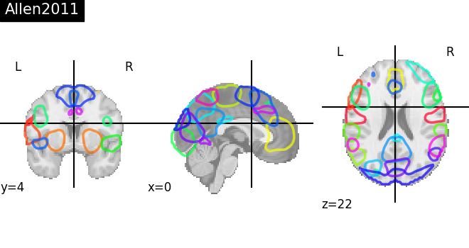
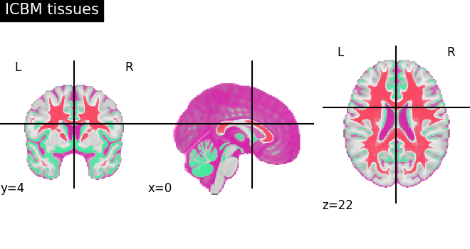
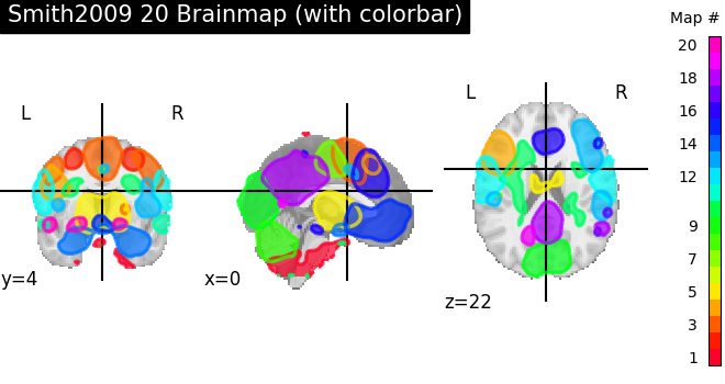
This example shows how to visualize probabilistic atlases made of 4D images. There are 3 different display types:

1. “contours”, which means maps or ROIs are shown as contours delineated by colored lines.

2. “filled_contours”, maps are shown as contours same as above but with fillings inside the contours.

3. “continuous”, maps are shown as just color overlays.

A colorbar can optionally be added.

The nilearn.plotting.plot_prob_atlas function displays each map with each different color which are picked randomly from the colormap which is already defined.

See Plotting brain images for more information to know how to tune the parameters.

Load 4D probabilistic atlases

from nilearn import datasets, plotting

# Allen RSN networks
allen = datasets.fetch_atlas_allen_2011()

# ICBM tissue probability
icbm = datasets.fetch_icbm152_2009()

# Smith ICA BrainMap 2009
smith_bm20 = datasets.fetch_atlas_smith_2009(resting=False, dimension=20)[
    "maps"
]

[get_dataset_dir] Dataset found in /home/remi/nilearn_data/allen_rsn_2011
[get_dataset_dir] Dataset found in /home/remi/nilearn_data/icbm152_2009
[get_dataset_dir] Dataset found in /home/remi/nilearn_data/smith_2009

Visualization

# "contours" example
plotting.plot_prob_atlas(allen.rsn28, title="Allen2011")

# "continuous" example
plotting.plot_prob_atlas(
    (icbm["wm"], icbm["gm"], icbm["csf"]), title="ICBM tissues"
)

# "filled_contours" example. An optional colorbar can be set.
plotting.plot_prob_atlas(
    smith_bm20,
    title="Smith2009 20 Brainmap (with colorbar)",
    colorbar=True,
)

plotting.show()

• 
• 
• 

/home/remi/github/nilearn/nilearn_doc_build/.tox/doc/lib/python3.9/site-packages/nilearn/plotting/displays/_axes.py:74: UserWarning: No contour levels were found within the data range.
  im = getattr(ax, type)(
/home/remi/github/nilearn/nilearn_doc_build/.tox/doc/lib/python3.9/site-packages/nilearn/plotting/displays/_axes.py:74: UserWarning: No contour levels were found within the data range.
  im = getattr(ax, type)(
/home/remi/github/nilearn/nilearn_doc_build/.tox/doc/lib/python3.9/site-packages/nilearn/plotting/displays/_axes.py:74: UserWarning: linewidths is ignored by contourf
  im = getattr(ax, type)(

Other probabilistic atlases accessible with nilearn

To save build time, the following code is not executed. Try running it locally to get the same plots as above for each of the listed atlases.

# Harvard Oxford Atlas
harvard_oxford = datasets.fetch_atlas_harvard_oxford("cort-prob-2mm")
harvard_oxford_sub = datasets.fetch_atlas_harvard_oxford("sub-prob-2mm")

# Smith ICA Atlas and Brain Maps 2009
smith_rsn10 = datasets.fetch_atlas_smith_2009(
    resting=True, dimension=10
)["maps"]
smith_rsn20 = datasets.fetch_atlas_smith_2009(
    resting=True, dimension=20
)["maps"]
smith_rsn70 = datasets.fetch_atlas_smith_2009(
    resting=True, dimension=70
)["maps"]
smith_bm10 = datasets.fetch_atlas_smith_2009(
    resting=False, dimension=10
)["maps"]
smith_bm70 = datasets.fetch_atlas_smith_2009(
    resting=False, dimension=70
)["maps"]

# Multi Subject Dictionary Learning Atlas
msdl = datasets.fetch_atlas_msdl()

# Pauli subcortical atlas
subcortex = datasets.fetch_atlas_pauli_2017()

# Dictionaries of Functional Modes (“DiFuMo”) atlas
dim = 64
res = 2
difumo = datasets.fetch_atlas_difumo(
    dimension=dim, resolution_mm=res, legacy_format=False
)

# Visualization
atlas_types = {
    "Harvard_Oxford": harvard_oxford.maps,
    "Harvard_Oxford sub": harvard_oxford_sub.maps,
    "Smith 2009 10 RSNs": smith_rsn10,
    "Smith2009 20 RSNs": smith_rsn20,
    "Smith2009 70 RSNs": smith_rsn70,
    "Smith2009 10 Brainmap": smith_bm10,
    "Smith2009 70 Brainmap": smith_bm70,
    "MSDL": msdl.maps,
    "Pauli2017 Subcortical Atlas": subcortex.maps,
    f"DiFuMo dimension {dim} resolution {res}": difumo.maps,
}

for name, atlas in sorted(atlas_types.items()):
    plotting.plot_prob_atlas(atlas, title=name)

plotting.show()

Estimated memory usage: 477 MB