Cortical surface-based searchlight decoding

This is a demo for surface-based searchlight decoding, as described in Chen et al.[1].

Warning

This example projects results from the Haxby dataset on the fsaverage surface. This is inappropriate given that the Haxby data has not been properly coregistered to allow for such projection. It is done in this example for pedagogical reasons to show “how to do it”.

Load Haxby dataset

import pandas as pd

from nilearn.datasets import fetch_haxby

# We fetch 2nd subject from haxby datasets (which is default)
haxby_dataset = fetch_haxby()

fmri_filename = haxby_dataset.func[0]
labels = pd.read_csv(haxby_dataset.session_target[0], sep=" ")
y = labels["labels"]
run = labels["chunks"]

[get_dataset_dir] Dataset found in /home/remi/nilearn_data/haxby2001

Restrict to faces and houses

from nilearn.image import index_img

condition_mask = y.isin(["face", "house"])

fmri_img = index_img(fmri_filename, condition_mask)
y, run = y[condition_mask], run[condition_mask]

Surface BOLD response

Fetch a coarse surface of the left hemisphere only for speed and average voxels 5 mm close to the 3d pial surface.

from sklearn import neighbors

from nilearn.datasets import load_fsaverage
from nilearn.surface import SurfaceImage

fsaverage = load_fsaverage()
fmri_img_surf = SurfaceImage.from_volume(
    mesh=fsaverage["pial"], volume_img=fmri_img, radius=5
)

Searchlight computation

import numpy as np
from sklearn.linear_model import RidgeClassifier
from sklearn.model_selection import KFold
from sklearn.pipeline import make_pipeline
from sklearn.preprocessing import StandardScaler

from nilearn.decoding.searchlight import search_light

# For the sake of speed,
# we will only run the decoding on one hemisphere
# in this example.
hemispheres_to_analyze = ["left"]
# Uncomment the following line if you want to run both hemispheres.
# hemispheres_to_analyze = ["left", "right"]

# Let us initialize a result scores dictionary ,
# to be able to create a SurfaceImage from it later.
scores = {
    "left": np.zeros(fmri_img_surf.mesh.parts["left"].n_vertices),
    "right": np.zeros(fmri_img_surf.mesh.parts["right"].n_vertices),
}

for hemi in hemispheres_to_analyze:
    print(f"Running searchlight on {hemi} hemisphere.")

    # To define the BOLD responses
    # to be included within each searchlight "sphere"
    # we define an adjacency matrix
    # based on the inflated surface vertices
    # such that nearby vertices are concatenated
    # within the same searchlight.
    coordinates = fsaverage["inflated"].parts[hemi].coordinates
    nn = neighbors.NearestNeighbors()
    adjacency = nn.fit(coordinates).radius_neighbors_graph(coordinates).tolil()

    # Simple linear estimator preceded by a normalization step
    estimator = make_pipeline(StandardScaler(), RidgeClassifier(alpha=10.0))

    # Define cross-validation scheme
    cv = KFold(n_splits=3, shuffle=False)

    X = fmri_img_surf.data.parts[hemi].T

    # Cross-validated search light
    scores[hemi] = search_light(
        X, y, estimator, adjacency, cv=cv, n_jobs=-1, verbose=1
    )

Running searchlight on left hemisphere.
[Parallel(n_jobs=-1)]: Using backend LokyBackend with 12 concurrent workers.
[Parallel(n_jobs=-1)]: Done   2 out of  12 | elapsed:   44.5s remaining:  3.7min
[Parallel(n_jobs=-1)]: Done  12 out of  12 | elapsed:   47.9s finished

Visualization

from nilearn.datasets import load_fsaverage_data
from nilearn.plotting import plot_surf_stat_map, show

fsaverage_data = load_fsaverage_data(mesh_type="inflated", data_type="sulcal")

score_img = SurfaceImage(mesh=fsaverage["inflated"], data=scores)

chance = 0.5
for hemi in hemispheres_to_analyze:
    score_img.data.parts[hemi] = score_img.data.parts[hemi] - chance

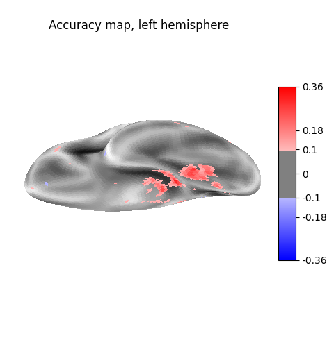
for hemi in hemispheres_to_analyze:
    plot_surf_stat_map(
        stat_map=score_img,
        view="ventral",
        hemi=hemi,
        colorbar=True,
        threshold=0.1,
        bg_map=fsaverage_data,
        title=f"Accuracy map, {hemi} hemisphere",
        cmap="bwr",
    )
show()

References

[1]

Yi Chen, Praneeth Namburi, Lloyd T. Elliott, Jakob Heinzle, Chun Siong Soon, Michael W.L. Chee, and John-Dylan Haynes. Cortical surface-based searchlight decoding. NeuroImage, 56(2):582–592, 2011. Multivariate Decoding and Brain Reading. URL: https://www.sciencedirect.com/science/article/pii/S1053811910010086, doi:https://doi.org/10.1016/j.neuroimage.2010.07.035.

Estimated memory usage: 1053 MB