Note
Go to the end to download the full example code or to run this example in your browser via Binder.
Encoding models for visual stimuli from Miyawaki et al. 2008
This example partly reproduces the encoding model presented in Miyawaki et al.[1].
Encoding models try to predict neuronal activity using information from presented stimuli, like an image or sound. Where decoding goes from brain data to real-world stimulus, encoding goes the other direction.
We demonstrate how to build such an encoding model in nilearn, predicting fMRI data from visual stimuli, using the dataset from Miyawaki et al.[1].
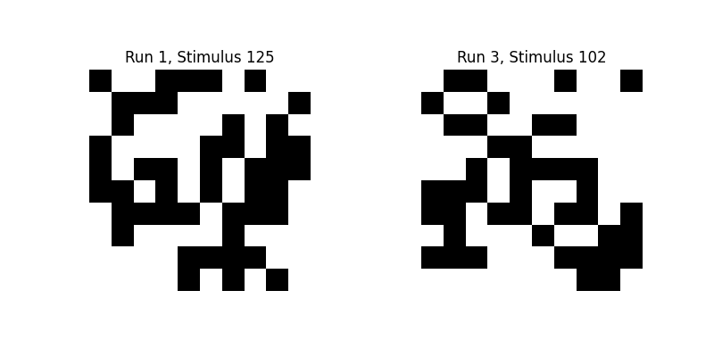
Participants were shown images, which consisted of random 10x10 binary (either black or white) pixels, and the corresponding fMRI activity was recorded. We will try to predict the activity in each voxel from the binary pixel-values of the presented images. Then we extract the receptive fields for a set of voxels to see which pixel location a voxel is most sensitive to.
See also
Reconstruction of visual stimuli from Miyawaki et al. 2008 for a decoding approach for the same dataset.
Warning
If you are using Nilearn with a version older than 0.9.0,
then you should either upgrade your version or import maskers
from the input_data module instead of the maskers module.
That is, you should manually replace in the following example all occurrences of:
from nilearn.maskers import NiftiMasker
with:
from nilearn.input_data import NiftiMasker
from nilearn._utils.helpers import check_matplotlib

check_matplotlib()

import matplotlib.pyplot as plt
Loading the data
Now we can load the data set:
from nilearn.datasets import fetch_miyawaki2008

dataset = fetch_miyawaki2008()
[fetch_miyawaki2008] Dataset created in /home/runner/nilearn_data/miyawaki2008
[fetch_miyawaki2008] Downloading data from
https://www.nitrc.org/frs/download.php/8486/miyawaki2008.tgz ...
[fetch_miyawaki2008] Downloaded 56606720 of 161069109 bytes (35.1%%,    1.9s
remaining)
[fetch_miyawaki2008] Downloaded 136519680 of 161069109 bytes (84.8%%,    0.4s
remaining)
[fetch_miyawaki2008]  ...done. (3 seconds, 0 min)

[fetch_miyawaki2008] Extracting data from
/home/runner/nilearn_data/miyawaki2008/8c2e6b1395a4722e90ce7d5fd40b6f09/miyawaki
2008.tgz...
[fetch_miyawaki2008] .. done.
We only use the training data of this study, where random binary images were shown.
# training data starts after the first 12 files
fmri_random_runs_filenames = dataset.func[12:]
stimuli_random_runs_filenames = dataset.label[12:]
We can use MultiNiftiMasker to load the fMRI
data, clean and mask it.
import numpy as np

from nilearn.maskers import MultiNiftiMasker

masker = MultiNiftiMasker(
    mask_img=dataset.mask,
    detrend=True,
    standardize="zscore_sample",
    n_jobs=2,
    verbose=1,
)
masker.fit()
fmri_data = masker.transform(fmri_random_runs_filenames)

# shape of the binary (i.e. black and white values) image in pixels
stimulus_shape = (10, 10)

# We load the visual stimuli from csv files
stimuli = [
    np.reshape(
        np.loadtxt(stimulus_run, dtype=int, delimiter=","),
        (-1, *stimulus_shape),
        order="F",
    )
    for stimulus_run in stimuli_random_runs_filenames
]
[MultiNiftiMasker.fit] Loading mask from
'/home/runner/nilearn_data/miyawaki2008/mask/mask.nii.gz'
/home/runner/work/nilearn/nilearn/examples/02_decoding/plot_miyawaki_encoding.py:69: UserWarning:

Data array used to create a new image contains 64-bit ints. This is likely due to creating the array with numpy and passing `int` as the `dtype`. Many tools such as FSL and SPM cannot deal with int64 in Nifti images, so for compatibility the data has been converted to int32.

[MultiNiftiMasker.fit] Resampling mask
[MultiNiftiMasker.fit] Finished fit
Let’s take a look at some of these binary images:
plt.figure(figsize=(8, 4))
plt.subplot(1, 2, 1)
plt.imshow(stimuli[0][124], interpolation="nearest", cmap="gray")
plt.axis("off")
plt.title("Run 1, Stimulus 125")
plt.subplot(1, 2, 2)
plt.imshow(stimuli[2][101], interpolation="nearest", cmap="gray")
plt.axis("off")
plt.title("Run 3, Stimulus 102")
plt.subplots_adjust(wspace=0.5)
We now stack the fMRI and stimulus data and remove an offset in the beginning/end.
fmri_data is a matrix of samples x voxels
print(f"{fmri_data.shape=}")
fmri_data.shape=(2860, 5438)
We flatten the last two dimensions of stimuli so it is a matrix of samples x pixels.
# Flatten the stimuli
stimuli = np.reshape(stimuli, (-1, stimulus_shape[0] * stimulus_shape[1]))

print(f"{stimuli.shape=}")
stimuli.shape=(2860, 100)
Building the encoding models
We can now proceed to build a simple voxel-wise encoding model using Ridge regression. For each voxel we fit an independent regression model, using the pixel-values of the visual stimuli to predict the neuronal activity in this voxel.
Using 10-fold cross-validation, we partition the data into 10 ‘folds’. We hold out each fold of the data for testing, then fit a ridge regression to the remaining 9/10 of the data, using stimuli as predictors and fmri_data as targets, and create predictions for the held-out 10th.
from sklearn.linear_model import Ridge
from sklearn.metrics import r2_score
from sklearn.model_selection import KFold

estimator = Ridge(alpha=100.0)
cv = KFold(n_splits=10)

scores = []
for train, test in cv.split(X=stimuli):
    # we train the Ridge estimator on the training set
    # and predict the fMRI activity for the test set
    predictions = estimator.fit(
        stimuli.reshape(-1, 100)[train], fmri_data[train]
    ).predict(stimuli.reshape(-1, 100)[test])
    # we compute how much variance our encoding model explains in each voxel
    scores.append(
        r2_score(fmri_data[test], predictions, multioutput="raw_values")
    )
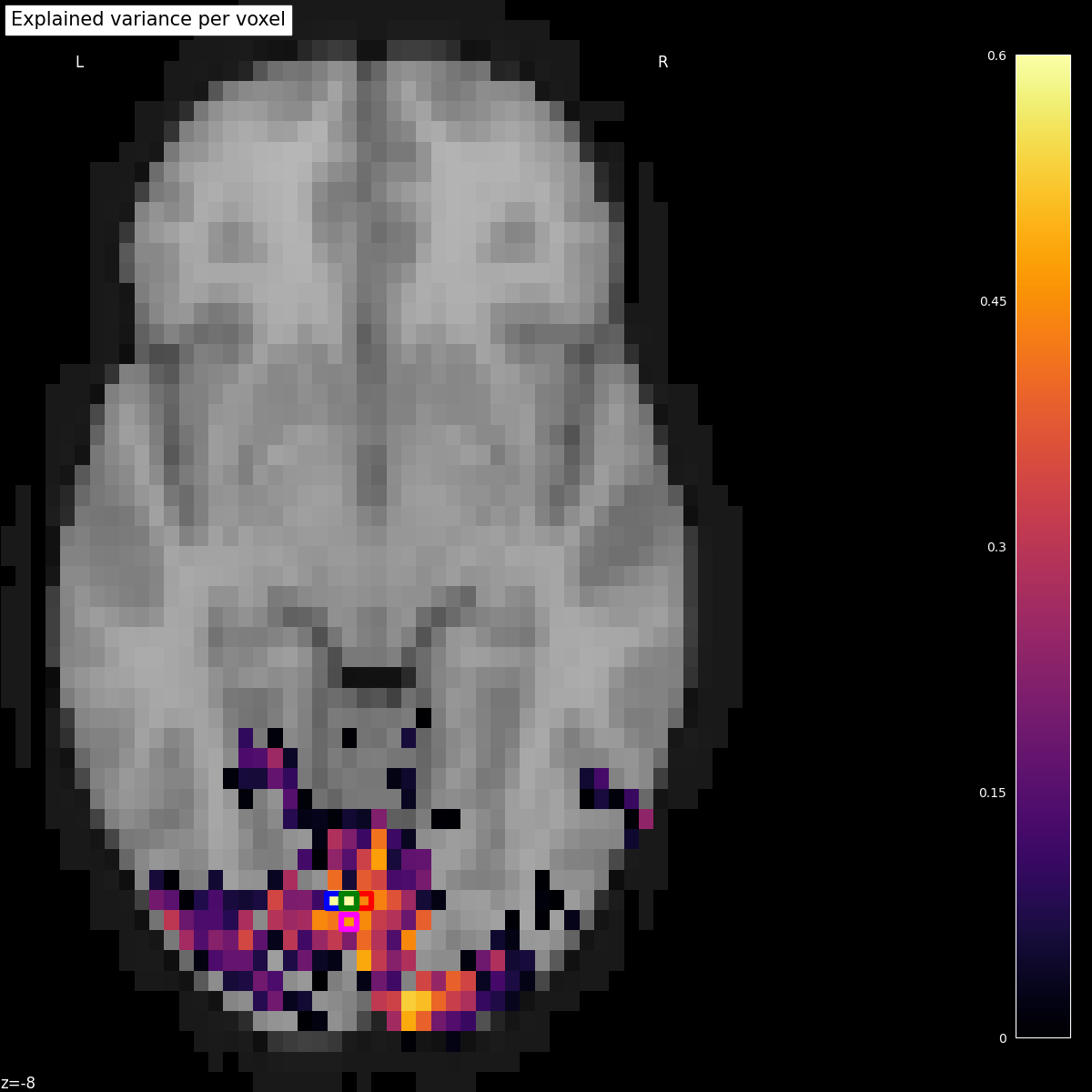
Mapping the encoding scores on the brain
To plot the scores onto the brain, we create a Nifti1Image containing the scores and then threshold it:
from nilearn.image import threshold_img

cut_score = np.mean(scores, axis=0)
cut_score[cut_score < 0] = 0

# bring the scores into the shape of the background brain
score_map_img = masker.inverse_transform(cut_score)

thresholded_score_map_img = threshold_img(
    score_map_img, threshold=1e-6, copy=False
)
[MultiNiftiMasker.inverse_transform] Computing image from signals
Plotting the statistical map on a background brain, we mark four voxels which we will inspect more closely later on.
from nilearn.image import coord_transform
from nilearn.plotting import plot_stat_map, show


def index_to_xy_coord(x, y, z=10):
    """Transform data index to coordinates of the background + offset."""
    coords = coord_transform(x, y, z, affine=thresholded_score_map_img.affine)
    return np.array(coords)[np.newaxis, :] + np.array([0, 1, 0])


xy_indices_of_special_voxels = [(30, 10), (32, 10), (31, 9), (31, 10)]

display = plot_stat_map(
    thresholded_score_map_img,
    bg_img=dataset.background,
    cut_coords=[-8],
    display_mode="z",
    aspect=1.25,
    title="Explained variance per voxel",
    cmap="inferno",
)

# creating a marker for each voxel and adding it to the statistical map

for i, (x, y) in enumerate(xy_indices_of_special_voxels):
    display.add_markers(
        index_to_xy_coord(x, y),
        marker_color="none",
        edgecolor=["b", "r", "magenta", "g"][i],
        marker_size=140,
        marker="s",
        facecolor="none",
        lw=4.5,
    )


# re-set figure size after construction so colorbar gets rescaled too
fig = plt.gcf()
fig.set_size_inches(12, 12)

show()
/home/runner/work/nilearn/nilearn/.tox/doc/lib/python3.10/site-packages/nilearn/plotting/displays/_slicers.py:994: UserWarning:

You passed both c and facecolor/facecolors for the markers. c has precedence over facecolor/facecolors. This behavior may change in the future.

/home/runner/work/nilearn/nilearn/examples/02_decoding/plot_miyawaki_encoding.py:217: UserWarning:

You are using the 'agg' matplotlib backend that is non-interactive.
No figure will be plotted when calling matplotlib.pyplot.show() or nilearn.plotting.show().
You can fix this by installing a different backend: for example via
        pip install PyQt6
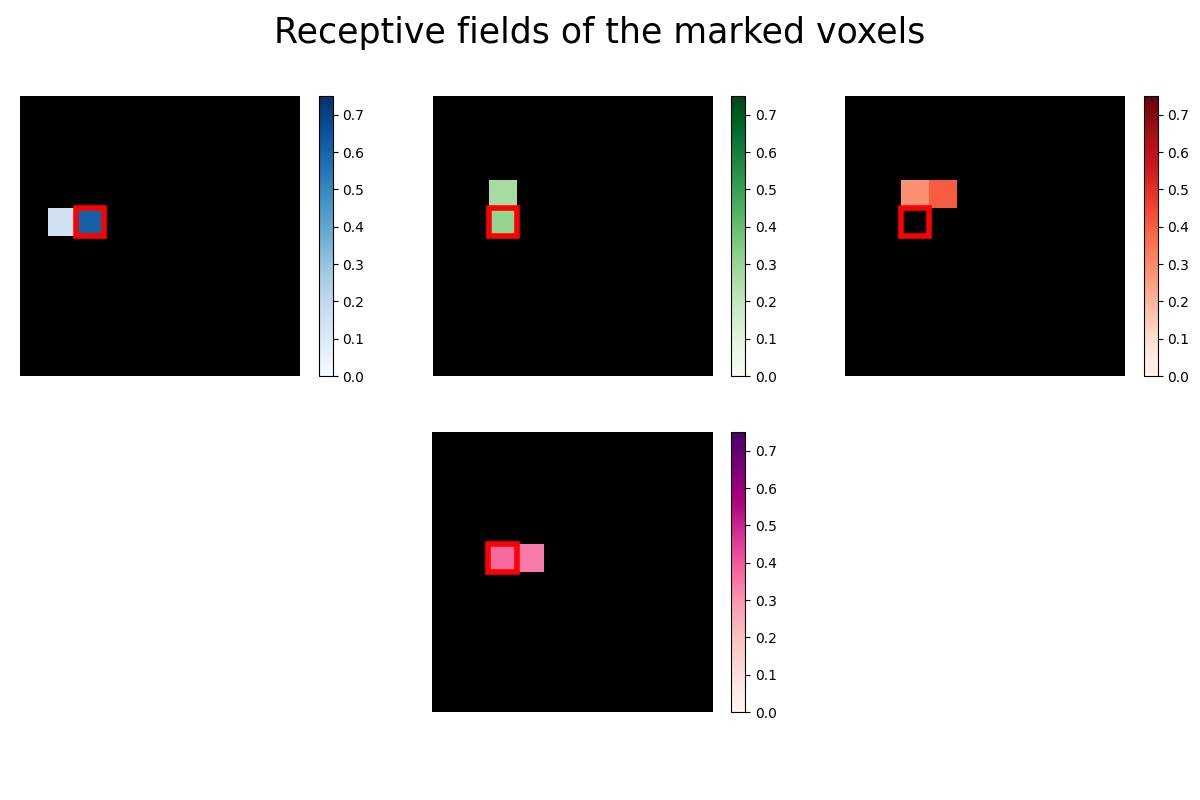
Estimating receptive fields
Now we take a closer look at the receptive fields of the four marked voxels. A voxel’s receptive field is the region of a stimulus (like an image) where the presence of an object, like a white instead of a black pixel, results in a change in activity in the voxel. In our case the receptive field is just the vector of 100 regression coefficients (one for each pixel) reshaped into the 10x10 form of the original images. Some voxels are receptive to only very few pixels, so we use Lasso regression to estimate a sparse set of regression coefficients.
from sklearn.linear_model import LassoLarsCV
from sklearn.pipeline import make_pipeline
from sklearn.preprocessing import StandardScaler

# automatically estimate the sparsity by cross-validation

lasso = make_pipeline(StandardScaler(), LassoLarsCV(max_iter=10))

# Mark the same pixel in each receptive field
marked_pixel = (4, 2)

from matplotlib import gridspec
from matplotlib.patches import Rectangle

fig = plt.figure(figsize=(12, 8))
fig.suptitle("Receptive fields of the marked voxels", fontsize=25)

# GridSpec allows us to do subplots with more control of the spacing
gs1 = gridspec.GridSpec(2, 3)

# we fit the Lasso for each of the three voxels of the upper row
for i, index in enumerate([1780, 1951, 2131]):
    ax = plt.subplot(gs1[0, i])
    lasso.fit(stimuli, fmri_data[:, index])
    # we reshape the coefficients into the form of the original images
    rf = lasso.named_steps["lassolarscv"].coef_.reshape((10, 10))
    # add a black background
    ax.imshow(np.zeros_like(rf), vmin=0.0, vmax=1.0, cmap="gray")
    ax_im = ax.imshow(
        np.ma.masked_less(rf, 0.1),
        interpolation="nearest",
        cmap=["Blues", "Greens", "Reds"][i],
        vmin=0.0,
        vmax=0.75,
    )
    # add the marked pixel
    ax.add_patch(
        Rectangle(
            (marked_pixel[1] - 0.5, marked_pixel[0] - 0.5),
            1,
            1,
            facecolor="none",
            edgecolor="r",
            lw=4,
        )
    )
    plt.axis("off")
    plt.colorbar(ax_im, ax=ax)

# and then for the voxel at the bottom

gs1.update(left=0.0, right=1.0, wspace=0.1)
ax = plt.subplot(gs1[1, 1])
lasso.fit(stimuli, fmri_data[:, 1935])
# we reshape the coefficients into the form of the original images
rf = lasso.named_steps["lassolarscv"].coef_.reshape((10, 10))
ax.imshow(np.zeros_like(rf), vmin=0.0, vmax=1.0, cmap="gray")
ax_im = ax.imshow(
    np.ma.masked_less(rf, 0.1),
    interpolation="nearest",
    cmap="RdPu",
    vmin=0.0,
    vmax=0.75,
)

# add the marked pixel
ax.add_patch(
    Rectangle(
        (marked_pixel[1] - 0.5, marked_pixel[0] - 0.5),
        1,
        1,
        facecolor="none",
        edgecolor="r",
        lw=4,
    )
)
plt.axis("off")
plt.colorbar(ax_im, ax=ax)
<matplotlib.colorbar.Colorbar object at 0x7f1f0cd81fc0>
The receptive fields of the four voxels are not only close to each other, the relative location of the pixel each voxel is most sensitive to roughly maps to the relative location of the voxels to each other. We can see a relationship between some voxel’s receptive field and its location in the brain.
References
Total running time of the script: (0 minutes 18.196 seconds)
Estimated memory usage: 497 MB