8.2. First level models

Page summary

First level models are, in essence, linear regression models run at the level of a single run or single subject. The model is applied on a voxel-wise basis, either on the whole brain or within a region of interest. The timecourse of each voxel is regressed against a predicted BOLD response created by convolving the haemodynamic response function (HRF) with a set of predictors defined within the design matrix.

8.2.1. HRF models

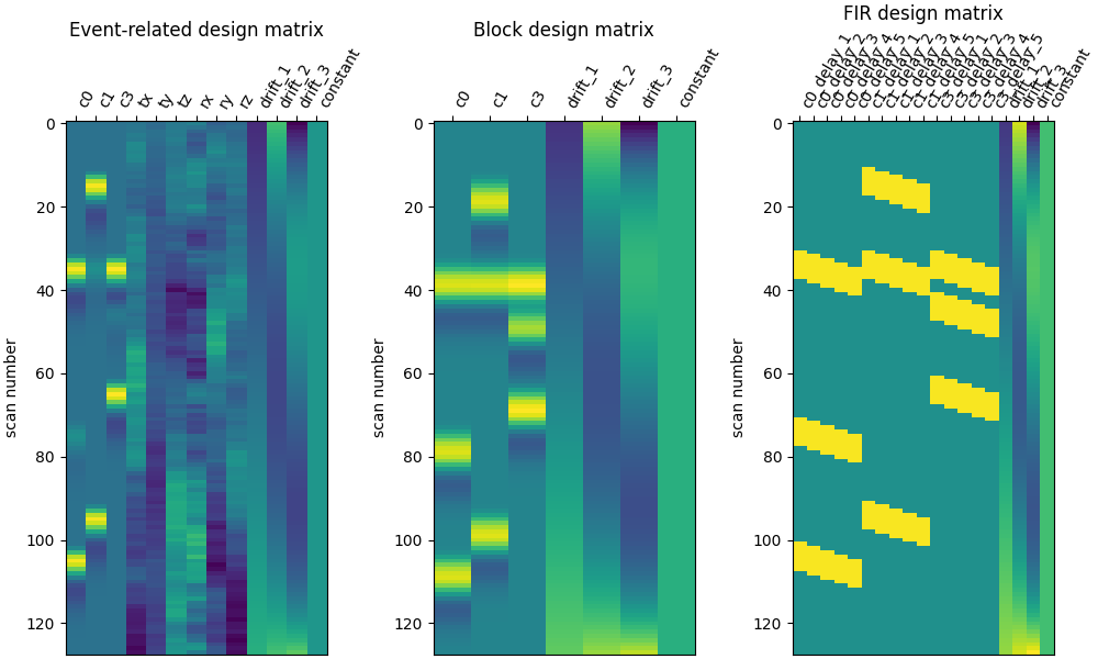
Nilearn offers a few different HRF models including the commonly used double-gamma SPM model (‘spm’) and the model shape proposed by G. Glover (‘glover’), both allowing the option of adding time and dispersion derivatives. The addition of these derivatives allows to better model any uncertainty in timing information. In addition, an FIR (finite impulse response, ‘fir’) model of the HRF is also available.

In order to visualize the predicted regressor prior to plugging it into the linear model, use the function nilearn.glm.first_level.compute_regressor, or explore the HRF plotting example Example of MRI response functions.

8.2.2. Design matrix: event-based and time series-based

8.2.2.1. Event-based

To create an event-based design matrix, information about the trial type, onset time and duration of the events in the experiment are necessary. This can be provided by the user, or be part of the dataset if using a BIDS-compatible dataset or one of the nilearn dataset fetcher functions like nilearn.datasets.fetch_spm_multimodal_fmri, nilearn.datasets.fetch_language_localizer_demo_dataset, etc.

Refer to the examples below for usage under the different scenarios:

• User-defined: Examples of design matrices

• Using an OpenNEURO dataset: First level analysis of a complete BIDS dataset from openneuro

• Using nilearn fetcher functions: Single-subject data (two runs) in native space

• Advanced beta series models: Beta-Series Modeling for Task-Based Functional Connectivity and Decoding

To ascertain that the sequence of events provided to the first level model is accurate, Nilearn provides an event visualization function called nilearn.plotting.plot_event. Sample usage for this is available in Generate an events.tsv file for the NeuroSpin localizer task.

Once the events are defined, the design matrix is created using the nilearn.glm.first_level.make_first_level_design_matrix function:

from nilearn.glm.first_level import make_first_level_design_matrix
design_matrices = make_first_level_design_matrix(frame_times, events,
                          drift_model='polynomial', drift_order=3)

Note

Additional predictors, like subject motion, can be specified using the add_reg parameter. Look at the function definition for available arguments.

A handy function called nilearn.plotting.plot_design_matrix can be used to visualize the design matrix. This is generally a good practice to follow before proceeding with the analysis:

from nilearn.plotting import plot_design_matrix
plot_design_matrix(design_matrices)

8.2.2.2. Time series-based

The time series of a seed region can also be used as the predictor for a first level model. This approach would help identify brain areas co-activating with the seed region. The time series is extracted using nilearn.maskers.NiftiSpheresMasker. For instance, if the seed region is the posterior cingulate cortex with coordinate [pcc_coords]:

from nilearn.maskers import NiftiSpheresMasker
seed_masker = NiftiSpheresMasker([pcc_coords], radius=10)
seed_time_series = seed_masker.fit_transform(adhd_dataset.func[0])

The seed_time_series is then passed into the design matrix using the add_reg argument mentioned in the note above. Code for this approach is in Default Mode Network extraction of ADHD dataset.

8.2.3. Fitting a first level model

The nilearn.glm.first_level.FirstLevelModel class provides the tools to fit the linear model to the fMRI data. The nilearn.glm.first_level.FirstLevelModel.fit function takes the fMRI data and design matrix as input and fits the GLM. Like other Nilearn functions, nilearn.glm.first_level.FirstLevelModel.fit accepts file names as input, but can also work with NiftiImage objects. More information about input formats is available here

from nilearn.glm.first_level import FirstLevelModel
fmri_glm = FirstLevelModel()
fmri_glm = fmri_glm.fit(subject_data, design_matrices=design_matrices)

8.2.3.1. Computing contrasts

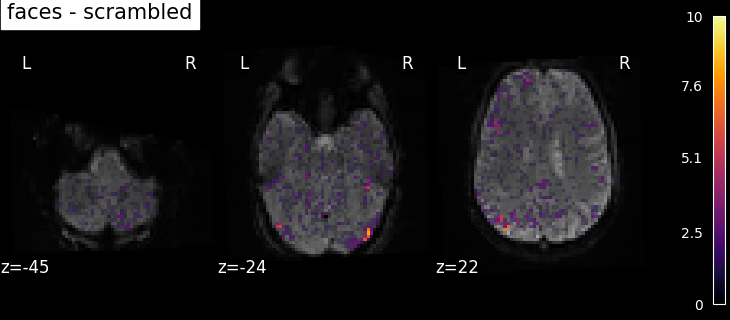
To get more interesting results out of the GLM model, contrasts can be computed between regressors of interest. The nilearn.glm.first_level.FirstLevelModel.compute_contrast function can be used for that. First, the contrasts of interest must be defined. In the spm_multimodal_fmri dataset referenced above, subjects are presented with ‘normal’ and ‘scrambled’ faces. The basic contrasts that can be constructed are the main effects of ‘normal faces’ and ‘scrambled faces’. Once the basic_contrasts have been set up, we can construct more interesting contrasts like ‘normal faces - scrambled faces’.

Note

The compute_contrast function can work with both numeric and symbolic arguments. See nilearn.glm.first_level.FirstLevelModel.compute_contrast for more information.

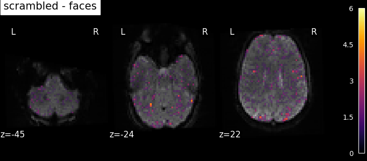
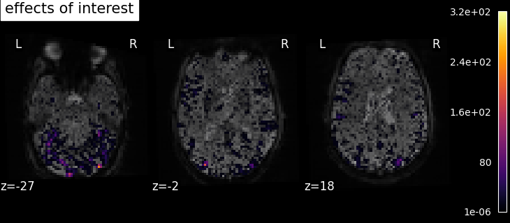
And finally we can compute the contrasts using the compute_contrast function. Refer to Single-subject data (two runs) in native space for the full example.

The activation maps from these 3 contrasts is presented below:

Additional example: Simple example of two-runs fMRI model fitting

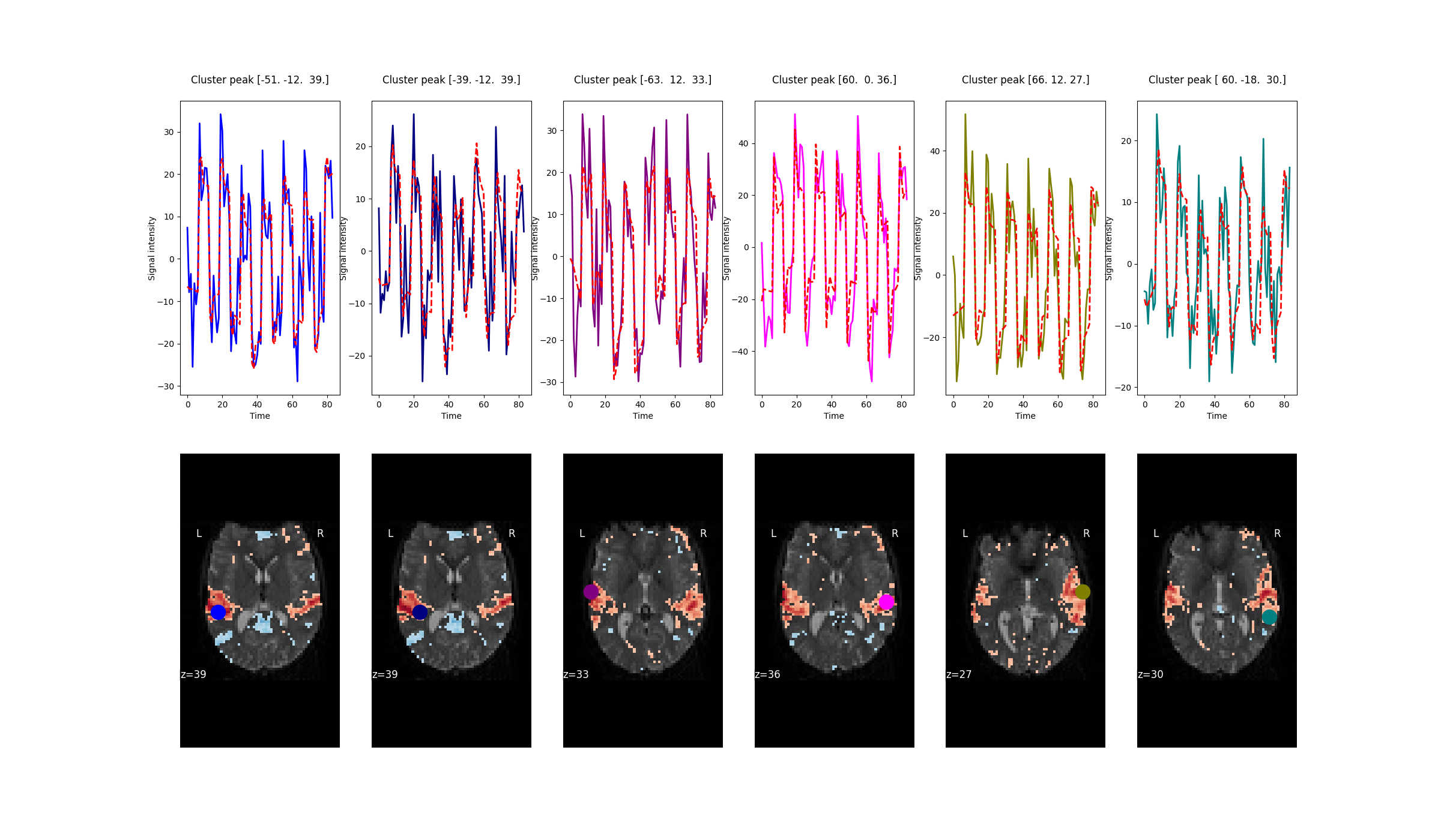
8.2.4. Extracting predicted time series and residuals

One way to assess the quality of the fit is to compare the observed and predicted time series of voxels. Nilearn makes the predicted time series easily accessible via a parameter called predicted that is part of the nilearn.glm.first_level.FirstLevelModel. This parameter is populated when FistLevelModel is initialized with the minimize_memory flag set to False.

observed_timeseries = masker.fit_transform(fmri_img)
predicted_timeseries = masker.fit_transform(fmri_glm.predicted[0])

Here, masker is an object of nilearn.maskers.NiftiSpheresMasker. In the figure below, predicted (red) and observed (not red) timecourses of 6 voxels are shown.

In addition to the predicted timecourses, this flag also yields the residuals of the GLM. The residuals are useful to calculate the F and R-squared statistic. For more information refer to Predicted time series and residuals

8.2.5. Surface-based analysis

fMRI analyses can also be performed on the cortical surface instead of a volumetric brain. Nilearn provides functions to map subject brains on to a cortical mesh, which can be either a standard surface as provided by, for e.g. Freesurfer, or a user-defined one. Freesurfer meshes can be accessed using nilearn.datasets.fetch_surf_fsaverage, while the function nilearn.surface.vol_to_surf does the projection from volumetric to surface space. Surface plotting functions like nilearn.plotting.plot_surf and nilearn.plotting.plot_surf_stat_map allow for easy visualization of surface-based data.

For a complete example refer to Example of surface-based first-level analysis