5.1. An introduction to decoding

This section gives an introduction to the main concept of decoding: predicting from brain images.

The discussion and examples are articulated on the analysis of the Haxby 2001 dataset, showing how to predict from fMRI images the stimuli that the subject is viewing. However the process is the same in other settings predicting from other brain imaging modalities, for instance predicting phenotype or diagnostic status from VBM (Voxel Based Morphometry) maps (as illustrated in a more complex example), or from FA maps to capture diffusion mapping.

Note

This documentation only aims at explaining the necessary concepts and common pitfalls of decoding analysis. For an introduction on the code to use please refer to : A introduction tutorial to fMRI decoding

5.1.1. Loading and preparing the data

5.1.1.1. The Haxby 2001 experiment

In the Haxby experiment, subjects were presented visual stimuli from different categories. We are going to predict which category the subject is seeing from the fMRI activity recorded in regions of the ventral visual system. Significant prediction shows that the signal in the region contains information on the corresponding category.

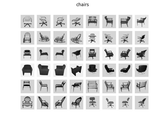
Face stimuli

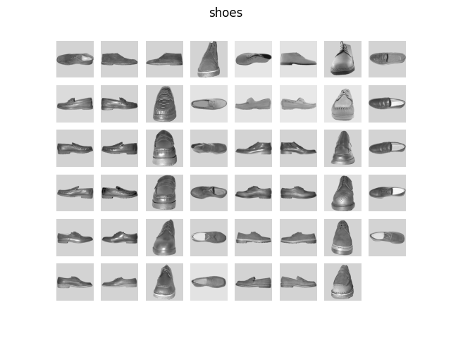
Cat stimuli

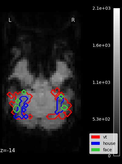
Masks

Decoding scores per mask

---

fMRI: using beta maps of a first-level analysis

The Haxby experiment is unusual because the experimental paradigm is made of many blocks of continuous stimulation. Most cognitive experiments have a more complex temporal structure with rich sequences of events (more on data input).

The standard approach to decoding consists in fitting a first-level general linear model (or GLM) to retrieve one response map (a beta map) per trial as shown in Decoding of a dataset after GLM fit for signal extraction. This is sometimes known as “beta-series regressions” (see Mumford et al.[1]). These maps can then be input to the decoder as below, predicting the conditions associated to trial.

For simplicity, we will work on the raw time-series of the data. However, it is strongly recommended that you fit a first-level model to include an hemodynamic response function (HRF) model and isolate the responses from various confounds as demonstrated in a more advanced example.

5.1.1.2. Loading the data into nilearn

Full code example

The documentation here just gives the big idea. A full code example, with explanation, can be found on A introduction tutorial to fMRI decoding

• Starting an environment: Launch IPython via “ipython –matplotlib” in a terminal, or use the Jupyter notebook.

• Retrieving the data: In the tutorial, we load the data using nilearn data downloading function, nilearn.datasets.fetch_haxby. However, all this function does is to download the data and return paths to the files downloaded on the disk. To input your own data to nilearn, you can pass in the path to your own files (more on data input).

• Masking fMRI data: To perform the analysis on some voxels only, we will provide a spatial mask of voxels to keep, which is provided with the dataset (here mask_vt a mask of the ventral temporal cortex that comes with data).

• Loading the behavioral labels: Behavioral information is often stored in a text file such as a CSV, and must be load with numpy.genfromtxt or pandas

• Sample mask: Masking some of the time points may be useful to restrict to a specific pair of conditions (eg cats versus faces).

See also

• Masking the data: from 4D image to 2D array To better control this process of spatial masking and add additional signal processing steps (smoothing, filtering, standardizing…), we could explicitly define a masker : nilearn.maskers.NiftiMasker. This object extracts voxels belonging to a given spatial mask and converts their signal to a 2D data matrix with a shape (n_timepoints, n_voxels) (see Masking data: from 4D Nifti images to 2D data arrays for a discussion on using masks).

Note

Seemingly minor data preparation can matter a lot on the final score, for instance standardizing the data.

5.1.2. Performing a simple decoding analysis

5.1.2.1. A few definitions

When doing predictive analysis you train an estimator to predict a variable of interest to you. Or in other words to predict a condition label y given a set X of imaging data.

This is always done in at least two steps:

• first a fit during which we “learn” the parameters of the model that make good predictions. This is done on some “training data” or “training set”.

• then a predict step where the “fitted” model is used to make prediction on new data. Here, we just have to give the new set of images (as the target should be unknown). These are called “test data” or “test set”.

All objects used to make prediction in Nilearn will at least have functions for these steps : a fit function and a predict function.

Warning

Do not predict on data used by the fit: this would yield misleadingly optimistic scores.

5.1.2.2. A first estimator

To perform decoding, we need a model that can learn some relations between X (the imaging data) and y the condition label. As a default, Nilearn uses Support Vector Classifier (or SVC) with a linear kernel. This is a simple yet performant choice that works in a wide variety of problems.

See also

The scikit-learn documentation on SVMs

5.1.2.3. Decoding made easy

Nilearn makes it easy to train a model with a principled pipeline using the nilearn.decoding.Decoder object. Using the mask we defined before and an SVC estimator as we already introduced, we can create a pipeline in two lines. The additional standardize=True argument adds a normalization of images signal to a zero mean and unit variance, which will improve performance of most estimators.

from nilearn.decoding import Decoder
decoder = Decoder(estimator='svc', mask=mask_filename)

Then we can fit it on the images and the conditions we chose before.

decoder.fit(fmri_niimgs, conditions)

This decoder can now be used to predict conditions for new images ! Be careful though, as we warned you, predicting on images that were used to fit your model should never be done.

5.1.2.4. Measuring prediction performance

One of the most common interests of decoding is to measure how well we can learn to predict various targets from our images to have a sense of which information is really contained in a given region of the brain. To do this, we need ways to measure the errors we make when we do prediction.

5.1.2.4.1. Cross-validation

We cannot measure prediction error on the same set of data that we have used to fit the estimator: it would be much easier than on new data, and the result would be meaningless. We need to use a technique called cross-validation to split the data into different sets, we can then fit our estimator on some set and measure an unbiased error on another set.

The easiest way to do cross-validation is the K-Fold strategy. If you do 5-fold cross-validation manually, you split your data in 5 folds, use 4 folds to fit your estimator, and 1 to predict and measure the errors made by your estimators. You repeat this for every combination of folds, and get 5 prediction “scores”, one for each fold.

During the fit, nilearn.decoding.Decoder object implicitly used a cross-validation: Stratified K-fold by default. You can easily inspect the prediction “score” it got in each fold.

print(decoder.cv_scores_)

5.1.2.4.2. Choosing a good cross-validation strategy

There are many cross-validation strategies possible, including K-Fold or leave-one-out. When choosing a strategy, keep in mind that the test set should be as little correlated as possible with the train set and have enough samples to enable a good measure the prediction error (at least 10-20% of the data as a rule of thumb).

As a general advice :

• To train a decoder on one subject data, try to leave at least one run out to have an independent test.

• To train a decoder across different subject data, leaving some subjects data out is often a good option.

• In any case leaving only one image as test set (leave-one-out) is often the worst option (see Varoquaux et al.[2]).

To improve our first pipeline for the Haxby example, we can leave one entire run out. To do this, we can pass a LeaveOneGroupOut cross-validation object from scikit-learn to our Decoder. Fitting it with the information of groups=`run_labels` will use one run as test set.

Note

Full code example can be found at : A introduction tutorial to fMRI decoding

5.1.2.4.3. Choice of the prediction accuracy measure

Once you have a prediction about new data and its real label (the ground truth) there are different ways to measure a score that summarizes its performance.

The default metric used for measuring errors is the accuracy score, i.e. the number of total errors. It is not always a sensible metric, especially in the case of very imbalanced classes, as in such situations choosing the dominant class can achieve a low number of errors.

Other metrics, such as the AUC (Area Under the Curve, for the ROC: the Receiver Operating Characteristic), can be used through the scoring argument of nilearn.decoding.Decoder.

See also

the list of scoring options

5.1.2.4.4. Prediction accuracy at chance using simple strategies

When performing decoding, prediction performance of a model can be checked against null distributions or random predictions. For this, we guess a chance level score using simple strategies while predicting condition y with X imaging data.

In Nilearn, we wrap Dummy estimators into the nilearn.decoding.Decoder that can be readily used to estimate this chance level score with the same model parameters that was previously used for real predictions. This allows us to compare whether the model is better than chance or not.

Putting it all together

The ROI-based decoding example does a decoding analysis per mask, giving the f1-score and chance score of the prediction for each object.

It uses all the notions presented above, with for loop to iterate over masks and categories and Python dictionaries to store the scores.

Masks

5.1.2.5. Visualizing the decoder’s weights

During fit step, the nilearn.decoding.Decoder object retains the coefficients of best models for each class in decoder.coef_img_.

Note

Full code for the above can be found on A introduction tutorial to fMRI decoding

See also

• Plotting brain images

5.1.3. Decoding without a mask: Anova-SVM

5.1.3.1. Dimension reduction with feature selection

If we do not start from a mask of the relevant regions, there is a very large number of voxels and not all are useful for face vs cat prediction. We thus add a feature selection procedure. The idea is to select the k voxels most correlated to the task through a simple F-score based feature selection (a.k.a. Anova)

You can directly choose to keep only a certain percentage of voxels in the nilearn.decoding.Decoder object through the screening_percentile argument. To keep the 10% most correlated voxels, just create us this parameter :

from nilearn.decoding import Decoder

# Here screening_percentile is set to 5 percent
mask_img = haxby_dataset.mask
decoder = Decoder(
    estimator="svc",
    mask=mask_img,
    smoothing_fwhm=4,
    standardize="zscore_sample",
    screening_percentile=5,
    scoring="accuracy",
)

# %%
# Fit the decoder and predict
# ---------------------------
decoder.fit(func_img, conditions)
y_pred = decoder.predict(func_img)

# %%
# Obtain prediction scores via cross validation
# ---------------------------------------------
# Define the cross-validation scheme used for validation. Here we use a
# LeaveOneGroupOut cross-validation on the run group which corresponds to a
# leave a run out scheme, then pass the cross-validator object
# to the cv parameter of decoder.leave-one-session-out.
# For more details please take a look at:
# `Measuring prediction scores using cross-validation\
# <../00_tutorials/plot_decoding_tutorial.html#measuring-prediction-scores-using-cross-validation>`_
from sklearn.model_selection import LeaveOneGroupOut

cv = LeaveOneGroupOut()

decoder = Decoder(
    estimator="svc",
    mask=mask_img,
    standardize="zscore_sample",
    screening_percentile=5,
    scoring="accuracy",
    cv=cv,
)
# Compute the prediction accuracy for the different folds (i.e. run)
decoder.fit(func_img, conditions, groups=run_label)

# Print the CV scores
print(decoder.cv_scores_["face"])

# %%

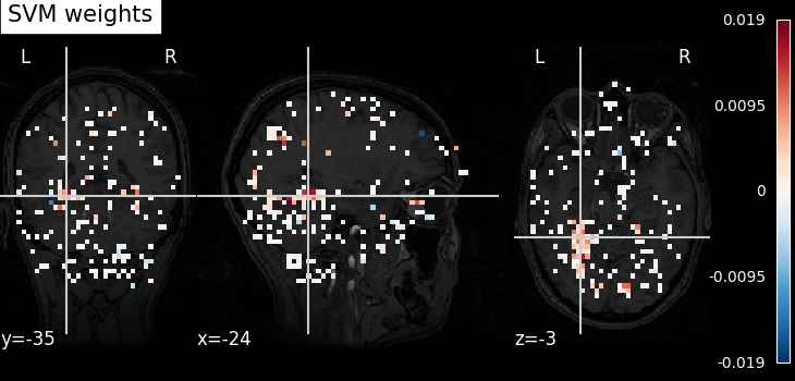
5.1.3.2. Visualizing the results

To visualize the results, nilearn.decoding.Decoder handles two main steps for you :

• first get the support vectors of the SVC and inverse the feature selection mechanism

• then, inverse the masking process to link weights to their spatial position and plot

# ---------------------
# Look at the SVC's discriminating weights using
# :class:`nilearn.plotting.plot_stat_map`
weight_img = decoder.coef_img_["face"]
from nilearn.plotting import plot_stat_map, show

plot_stat_map(weight_img, bg_img=haxby_dataset.anat[0], title="SVM weights")

show()
# %%
# Or we can plot the weights using :class:`nilearn.plotting.view_img` as a
# dynamic html viewer
from nilearn.plotting import view_img

view_img(weight_img, bg_img=haxby_dataset.anat[0], title="SVM weights", dim=-1)
# %%

See also

• Plotting brain images

Final script

The complete script to do an SVM-Anova analysis can be found as an example.

See also

• FREM: fast ensembling of regularized models for robust decoding

• SpaceNet: decoding with spatial structure for better maps

• Searchlight : finding voxels containing information

5.1.3.3. References

[1]

Jeanette A Mumford, Benjamin O Turner, F Gregory Ashby, and Russell A Poldrack. Deconvolving bold activation in event-related designs for multivoxel pattern classification analyses. Neuroimage, 59(3):2636–2643, 2012.

[2]

Gaël Varoquaux, Pradeep Reddy Raamana, Denis A Engemann, Andrés Hoyos-Idrobo, Yannick Schwartz, and Bertrand Thirion. Assessing and tuning brain decoders: cross-validation, caveats, and guidelines. NeuroImage, 145:166–179, 2017. arXiv:https://arxiv.org/pdf/1606.05201.pdf.