Note
Go to the end to download the full example code. or to run this example in your browser via Binder
The Haxby dataset: different multi-class strategies
In this example,
we compare one vs all and one vs one multi-class strategies:
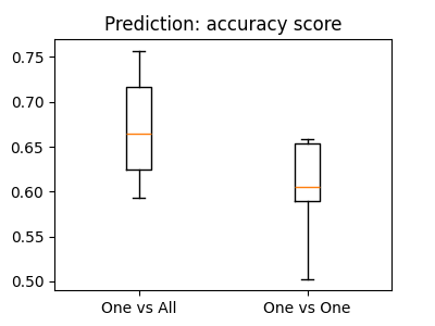
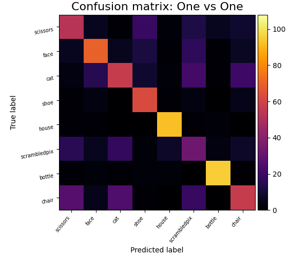
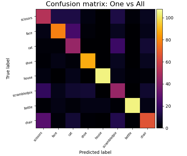
We compare their overall cross-validated accuracy and their confusion matrix.
See the scikit-learn documentation about multiclass classification.
import numpy as np
import pandas as pd

from nilearn import datasets
Load and prepare the Haxby dataset
By default 2nd subject from haxby datasets will be fetched.
haxby_dataset = datasets.fetch_haxby()

func_filename = haxby_dataset.func[0]
mask_filename = haxby_dataset.mask

print(f"Mask nifti images are located at: {mask_filename}")
print(f"Functional nifti images are located at: {func_filename}")
[fetch_haxby] Dataset directory found: /home/runner/work/nilearn/nilearn/nilearn_data/haxby2001
Mask nifti images are located at: /home/runner/work/nilearn/nilearn/nilearn_data/haxby2001/mask.nii.gz
Functional nifti images are located at: /home/runner/work/nilearn/nilearn/nilearn_data/haxby2001/subj2/bold.nii.gz
We load the behavioral data that we will predict and
remove the "rest" condition, as it is of no interest to us.
See also
For more information about the dataset see its description.
We extract the data with a NiftiMasker.
For decoding, standardizing is often very important,
so we set standardize="zscore_sample".
from nilearn.maskers import NiftiMasker

nifti_masker = NiftiMasker(
    mask_img=mask_filename,
    runs=run,
    smoothing_fwhm=4,
    standardize="zscore_sample",
    memory="nilearn_cache",
    memory_level=1,
    verbose=1,
)
X = nifti_masker.fit_transform(func_filename)
[NiftiMasker.wrapped] Loading data from .../subj2/bold.nii.gz
[NiftiMasker.wrapped] Loading mask from .../mask.nii.gz
[NiftiMasker.wrapped] Resampling mask
[NiftiMasker.wrapped] Finished fit
________________________________________________________________________________
[Memory] Calling nilearn.maskers.nifti_masker.filter_and_mask...
filter_and_mask('/home/runner/work/nilearn/nilearn/nilearn_data/haxby2001/subj2/bold.nii.gz', <nibabel.nifti1.Nifti1Image object at 0x7f2da0cefb20>, { 'clean_args': None,
  'clean_kwargs': {},
  'cmap': 'gray',
  'detrend': False,
  'dtype': None,
  'high_pass': None,
  'high_variance_confounds': False,
  'low_pass': None,
  'reports': True,
  'runs': 0        0
1        0
2        0
3        0
4        0
        ..
1447    11
1448    11
1449    11
1450    11
1451    11
Name: chunks, Length: 1452, dtype: int64,
  'smoothing_fwhm': 4,
  'standardize': 'zscore_sample',
  'standardize_confounds': True,
  't_r': None,
  'target_affine': None,
  'target_shape': None}, memory_level=1, memory=Memory(location=nilearn_cache/joblib), verbose=1, confounds=None, sample_mask=None, copy=True, sklearn_output_config=None)
[NiftiMasker.wrapped] Loading data from <nibabel.nifti1.Nifti1Image object at 0x7f2da0cede10>
[NiftiMasker.wrapped] Smoothing images
[NiftiMasker.wrapped] Extracting region signals
[NiftiMasker.wrapped] Cleaning extracted signals
_________________________________________________filter_and_mask - 10.7s, 0.2min
Remove the "rest" condition
Build the decoders, using scikit-learn
Nilearn does not have dedicated multiclass estimators,
as we can directly use those from sklearn.
Here we use a Support Vector Classification (sklearn.svm.SVC),
with a linear kernel, and a simple feature selection step.
from sklearn.feature_selection import SelectKBest, f_classif
from sklearn.multiclass import OneVsOneClassifier, OneVsRestClassifier
from sklearn.pipeline import Pipeline
from sklearn.svm import SVC
svc_ovo = OneVsOneClassifier(
    Pipeline(
        [
            ("anova", SelectKBest(f_classif, k=500)),
            ("svc", SVC(kernel="linear")),
        ]
    )
)
svc_ovo
svc_ova = OneVsRestClassifier(
    Pipeline(
        [
            ("anova", SelectKBest(f_classif, k=500)),
            ("svc", SVC(kernel="linear")),
        ]
    )
)
svc_ova
Now we compute cross-validation scores
The fMRI data is acquired by runs, and the noise is autocorrelated in a given run. Hence, it is better to predict across runs when doing cross-validation. Here we do a 5 fold cross-validation.
from sklearn.model_selection import cross_val_score

cv = 5
cv_scores_ovo = cross_val_score(svc_ovo, X, y, cv=cv, verbose=1)
cv_scores_ovo
[Parallel(n_jobs=1)]: Using backend SequentialBackend with 1 concurrent workers.
[Parallel(n_jobs=1)]: Done   5 out of   5 | elapsed:    9.2s finished

array([0.50289017, 0.65895954, 0.58959538, 0.65317919, 0.60465116])
cv_scores_ova = cross_val_score(svc_ova, X, y, cv=cv, verbose=1)
cv_scores_ova
[Parallel(n_jobs=1)]: Using backend SequentialBackend with 1 concurrent workers.
[Parallel(n_jobs=1)]: Done   5 out of   5 | elapsed:    4.8s finished

array([0.62427746, 0.71676301, 0.66473988, 0.75722543, 0.59302326])
print("OvO:", cv_scores_ovo.mean().round(decimals=3))
print("OvA:", cv_scores_ova.mean().round(decimals=3))
OvO: 0.602
OvA: 0.671
Plot barplots of the prediction scores
from matplotlib import pyplot as plt

from nilearn.plotting import show

plt.figure(figsize=(4, 3))
plt.boxplot([cv_scores_ova, cv_scores_ovo])
plt.xticks([1, 2], ["One vs All", "One vs One"])
plt.title("Prediction: accuracy score")

show()
Plot the cross-validated confusion matrices
Instead of fitting on a single train/test split, we use
sklearn.model_selection.cross_val_predict with the same
cross-validation as above to get, for each sample,
a prediction made by a model that never saw that sample during training.
We can then build a single confusion matrix from those out-of-fold
predictions for the whole dataset.
from sklearn.model_selection import cross_val_predict

y_pred_ovo = cross_val_predict(svc_ovo, X, y, cv=cv, verbose=1)

y_pred_ova = cross_val_predict(svc_ova, X, y, cv=cv, verbose=1)
[Parallel(n_jobs=1)]: Using backend SequentialBackend with 1 concurrent workers.
[Parallel(n_jobs=1)]: Done   5 out of   5 | elapsed:    9.4s finished
[Parallel(n_jobs=1)]: Using backend SequentialBackend with 1 concurrent workers.
[Parallel(n_jobs=1)]: Done   5 out of   5 | elapsed:    4.8s finished
We get the labels of the numerical conditions represented by the vector y and we sort the conditions by the order of appearance.
from sklearn.metrics import confusion_matrix

from nilearn.plotting import plot_matrix

unique_conditions, order = np.unique(y, return_index=True)
unique_conditions = unique_conditions[np.argsort(order)]

im = plot_matrix(
    confusion_matrix(y_pred_ovo, y),
    labels=unique_conditions,
    title="Confusion matrix: One vs One",
    cmap="inferno",
    figure=(6, 5),
    auto_fit=False,
    vmax=108,
)
ax = im.axes
ax.set_ylabel("True label")
ax.set_xlabel("Predicted label")

im = plot_matrix(
    confusion_matrix(y_pred_ova, y),
    labels=unique_conditions,
    title="Confusion matrix: One vs All",
    cmap="inferno",
    figure=(6, 5),
    auto_fit=False,
    vmax=108,
)
ax = im.axes
ax.set_ylabel("True label")
ax.set_xlabel("Predicted label")

show()
Total running time of the script: (0 minutes 44.699 seconds)
Estimated memory usage: 2572 MB
