Note
Click here to download the full example code or to run this example in your browser via Binder
9.2.18. Glass brain plotting in nilearn (all options)
First part of this example goes through different options of the
nilearn.plotting.plot_glass_brain function (including plotting
negative values).
Second part, goes through same options but selected of the same glass brain function but plotting is seen with contours.
See Plotting brain images for more plotting functionalities and Section 4.3 for more details about display objects in Nilearn.
Also, see nilearn.datasets.fetch_neurovault_motor_task for details
about the plotting data and associated meta-data.
9.2.18.1. Retrieve the data
Nilearn comes with set of functions that download public data from Internet
Let us first see where the data will be downloded and stored on our disk:
from nilearn import datasets
print('Datasets shipped with nilearn are stored in: %r' % datasets.get_data_dirs())
Out:
Datasets shipped with nilearn are stored in: ['/home/nicolas/nilearn_data']
Let us now retrieve a motor task contrast map corresponding to a group one-sample t-test
motor_images = datasets.fetch_neurovault_motor_task()
stat_img = motor_images.images[0]
# stat_img is just the name of the file that we downloded
stat_img
Out:
'/home/nicolas/nilearn_data/neurovault/collection_658/image_10426.nii.gz'
9.2.18.2. Demo glass brain plotting
from nilearn import plotting

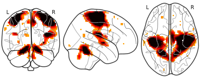
# Whole brain sagittal cuts and map is thresholded at 3
plotting.plot_glass_brain(stat_img, threshold=3)
Out:
<nilearn.plotting.displays.OrthoProjector object at 0x7fc6aae0aa00>
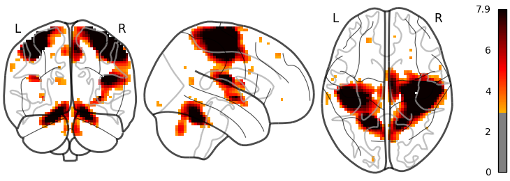
With a colorbar
plotting.plot_glass_brain(stat_img, threshold=3, colorbar=True)
Out:
<nilearn.plotting.displays.OrthoProjector object at 0x7fc6a823a5e0>
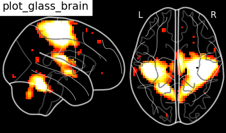
Black background, and only the (x, z) cuts
plotting.plot_glass_brain(stat_img, title='plot_glass_brain',
                          black_bg=True, display_mode='xz', threshold=3)
Out:
<nilearn.plotting.displays.XZProjector object at 0x7fc6a3efe5b0>
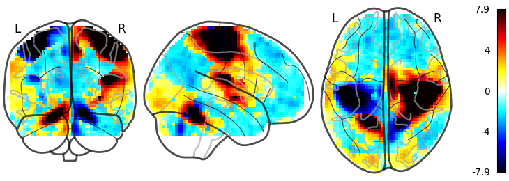
Plotting the sign of the activation with plot_abs to False
plotting.plot_glass_brain(stat_img, threshold=0, colorbar=True,
                          plot_abs=False)
Out:
<nilearn.plotting.displays.OrthoProjector object at 0x7fc6a3b5fe20>
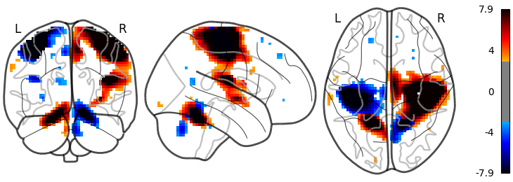
The sign of the activation and a colorbar
plotting.plot_glass_brain(stat_img, threshold=3,
                          colorbar=True, plot_abs=False)
Out:
<nilearn.plotting.displays.OrthoProjector object at 0x7fc6a2f18f70>
9.2.18.3. Different projections for the left and right hemispheres
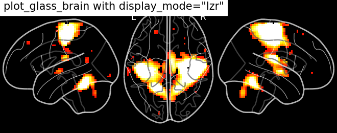
Hemispheric sagittal cuts
plotting.plot_glass_brain(stat_img,
                          title='plot_glass_brain with display_mode="lzr"',
                          black_bg=True, display_mode='lzr', threshold=3)
Out:
<nilearn.plotting.displays.LZRProjector object at 0x7fc6a34ea5b0>
plotting.plot_glass_brain(stat_img, threshold=0, colorbar=True,
                          title='plot_glass_brain with display_mode="lyrz"',
                          plot_abs=False, display_mode='lyrz')

Out:
<nilearn.plotting.displays.LYRZProjector object at 0x7fc69243da30>
9.2.18.4. Demo glass brain plotting with contours and with fillings
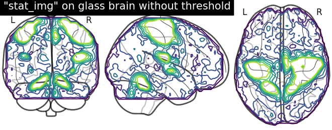
To plot maps with contours, we call the plotting function into variable from which we can use specific display features which are inherited automatically. In this case, we focus on using add_contours First, we initialize the plotting function into “display” and first argument set to None since we want an empty glass brain to plotting the statistical maps with “add_contours”
display = plotting.plot_glass_brain(None)
# Here, we project statistical maps
display.add_contours(stat_img)
# and a title
display.title('"stat_img" on glass brain without threshold')
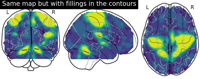
Plotting with filled=True implies contours with fillings. Here, we are not specifying levels
display = plotting.plot_glass_brain(None)
# Here, we project statistical maps with filled=True
display.add_contours(stat_img, filled=True)
# and a title
display.title('Same map but with fillings in the contours')
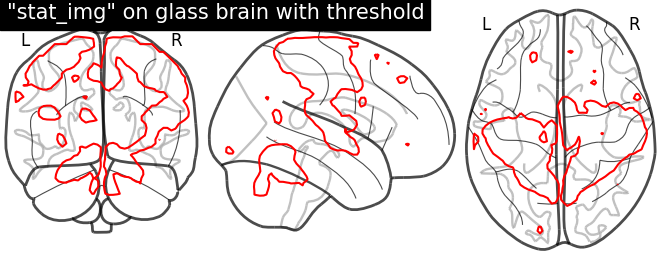
Here, we input specific level (cut-off) in the statistical map. In other way, we are thresholding our statistical map
# Here, we set the threshold using parameter called `levels` with value given
# in a list and choosing color to Red.
display = plotting.plot_glass_brain(None)
display.add_contours(stat_img, levels=[3.], colors='r')
display.title('"stat_img" on glass brain with threshold')
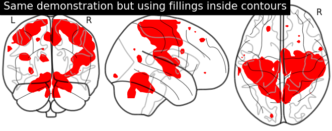
Plotting with same demonstration but inlcudes now filled=True
display = plotting.plot_glass_brain(None)
display.add_contours(stat_img, filled=True, levels=[3.], colors='r')
display.title('Same demonstration but using fillings inside contours')
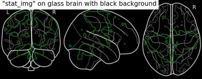
Plotting with black background, black_bg should be set with plot_glass_brain
# We can set black background using black_bg=True
display = plotting.plot_glass_brain(None, black_bg=True)
display.add_contours(stat_img, levels=[3.], colors='g')
display.title('"stat_img" on glass brain with black background')
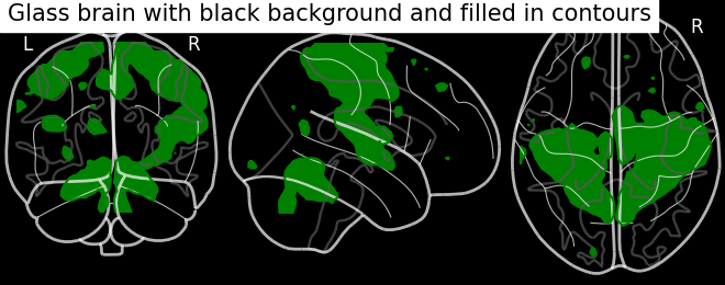
Black background plotting with filled in contours
display = plotting.plot_glass_brain(None, black_bg=True)
display.add_contours(stat_img, filled=True, levels=[3.], colors='g')
display.title('Glass brain with black background and filled in contours')
9.2.18.5. Display contour projections in both hemispheres
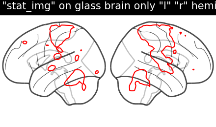
Key argument to vary here is display_mode for hemispheric plotting
# Now, display_mode is chosen as 'lr' for both hemispheric plots
display = plotting.plot_glass_brain(None, display_mode='lr')
display.add_contours(stat_img, levels=[3.], colors='r')
display.title('"stat_img" on glass brain only "l" "r" hemispheres')
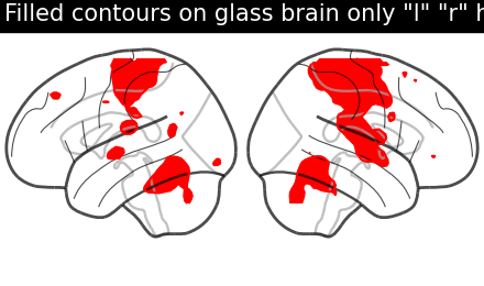
Filled contours in both hemispheric plotting, just by adding filled=True
display = plotting.plot_glass_brain(None, display_mode='lr')
display.add_contours(stat_img, filled=True, levels=[3.], colors='r')
display.title('Filled contours on glass brain only "l" "r" hemispheres')
With positive and negative sign of activations with plot_abs in plot_glass_brain
# By default parameter `plot_abs` is True and sign of activations can be
# displayed by changing `plot_abs` to False
display = plotting.plot_glass_brain(None, plot_abs=False, display_mode='lzry')
display.add_contours(stat_img)
display.title("Contours with both sign of activations without threshold")

Now, adding just filled=True to get positive and negative sign activations with fillings in the contours
display = plotting.plot_glass_brain(None, plot_abs=False, display_mode='lzry')
display.add_contours(stat_img, filled=True)
display.title("Filled contours with both sign of activations without threshold")

Displaying both signs (positive and negative) of activations with threshold meaning thresholding by adding an argument levels in add_contours.
import numpy as np
display = plotting.plot_glass_brain(None, plot_abs=False, display_mode='lzry')

# In add_contours,
# we give two values through the argument `levels` which corresponds to the
# thresholds of the contour we want to draw: One is positive and the other one
# is negative. We give a list of `colors` as argument to associate a different
# color to each contour. Additionally, we also choose to plot contours with
# thick line widths, For linewidths one value would be enough so that same
# value is used for both contours.
display.add_contours(stat_img, levels=[-2.8, 3.], colors=['b', 'r'],
                     linewidths=4.)
display.title('Contours with sign of activations with threshold')

Same display demonstration as above but just adding filled=True to get fillings inside the contours.
# Unlike in previous plot, here we specify each sign at a time. We call negative
# values display first followed by positive values display.

# First, we fetch our display object with same parametes used as above
display = plotting.plot_glass_brain(None, plot_abs=False, display_mode='lzry')

# Second, we plot negative sign of activation with levels given as negative
# activation value in a list. Upper bound should be kept to -infinity
display.add_contours(stat_img, filled=True, levels=[-np.inf, -2.8],
                     colors='b')
# Next, within same plotting object we plot positive sign of activation
display.add_contours(stat_img, filled=True, levels=[3.], colors='r')
display.title('Now same plotting but with filled contours')

# Finally, displaying them
plotting.show()

Total running time of the script: ( 0 minutes 19.603 seconds)
