9.4.1. Extracting signals of a probabilistic atlas of functional regions

This example extracts the signal on regions defined via a probabilistic atlas, to construct a functional connectome.

We use the MSDL atlas of functional regions in movie-watching.

The key to extract signals is to use the nilearn.input_data.NiftiMapsMasker that can transform nifti objects to time series using a probabilistic atlas.

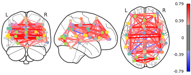
As the MSDL atlas comes with (x, y, z) MNI coordinates for the different regions, we can visualize the matrix as a graph of interaction in a brain. To avoid having too dense a graph, we represent only the 20% edges with the highest values.

9.4.1.1. Retrieve the atlas and the data

from nilearn import datasets
atlas = datasets.fetch_atlas_msdl()
# Loading atlas image stored in 'maps'
atlas_filename = atlas['maps']
# Loading atlas data stored in 'labels'
labels = atlas['labels']

# Load the functional datasets
data = datasets.fetch_development_fmri(n_subjects=1)

print('First subject resting-state nifti image (4D) is located at: %s' %
      data.func[0])

Out:

/home/nicolas/anaconda3/envs/nilearn/lib/python3.8/site-packages/numpy/lib/npyio.py:2405: VisibleDeprecationWarning: Reading unicode strings without specifying the encoding argument is deprecated. Set the encoding, use None for the system default.
  output = genfromtxt(fname, **kwargs)
First subject resting-state nifti image (4D) is located at: /home/nicolas/nilearn_data/development_fmri/development_fmri/sub-pixar123_task-pixar_space-MNI152NLin2009cAsym_desc-preproc_bold.nii.gz

9.4.1.2. Extract the time series

from nilearn.input_data import NiftiMapsMasker
masker = NiftiMapsMasker(maps_img=atlas_filename, standardize=True,
                         memory='nilearn_cache', verbose=5)

time_series = masker.fit_transform(data.func[0],
                                   confounds=data.confounds)

Out:

[NiftiMapsMasker.fit_transform] loading regions from /home/nicolas/nilearn_data/msdl_atlas/MSDL_rois/msdl_rois.nii
Resampling maps
/home/nicolas/GitRepos/nilearn-fork/nilearn/_utils/cache_mixin.py:303: UserWarning: memory_level is currently set to 0 but a Memory object has been provided. Setting memory_level to 1.
  warnings.warn("memory_level is currently set to 0 but "
________________________________________________________________________________
[Memory] Calling nilearn.image.resampling.resample_img...
resample_img(<nibabel.nifti1.Nifti1Image object at 0x7f881e682be0>, interpolation='continuous', target_shape=(50, 59, 50), target_affine=array([[   4.,    0.,    0.,  -96.],
       [   0.,    4.,    0., -132.],
       [   0.,    0.,    4.,  -78.],
       [   0.,    0.,    0.,    1.]]))
_____________________________________________________resample_img - 1.6s, 0.0min
________________________________________________________________________________
[Memory] Calling nilearn.input_data.base_masker.filter_and_extract...
filter_and_extract('/home/nicolas/nilearn_data/development_fmri/development_fmri/sub-pixar123_task-pixar_space-MNI152NLin2009cAsym_desc-preproc_bold.nii.gz',
<nilearn.input_data.nifti_maps_masker._ExtractionFunctor object at 0x7f881e5b8ac0>,
{ 'allow_overlap': True,
  'detrend': False,
  'dtype': None,
  'high_pass': None,
  'high_variance_confounds': False,
  'low_pass': None,
  'maps_img': '/home/nicolas/nilearn_data/msdl_atlas/MSDL_rois/msdl_rois.nii',
  'mask_img': None,
  'smoothing_fwhm': None,
  'standardize': True,
  'standardize_confounds': True,
  't_r': None,
  'target_affine': None,
  'target_shape': None}, confounds=[ '/home/nicolas/nilearn_data/development_fmri/development_fmri/sub-pixar123_task-pixar_desc-reducedConfounds_regressors.tsv'], dtype=None, memory=Memory(location=nilearn_cache/joblib), memory_level=1, verbose=5)
[NiftiMapsMasker.transform_single_imgs] Loading data from /home/nicolas/nilearn_data/development_fmri/development_fmri/sub-pixar123_task-pixar_space-MNI152NLin2009cAsym_desc-preproc_bold.nii.gz
[NiftiMapsMasker.transform_single_imgs] Extracting region signals
[NiftiMapsMasker.transform_single_imgs] Cleaning extracted signals
_______________________________________________filter_and_extract - 2.3s, 0.0min

time_series is now a 2D matrix, of shape (number of time points x number of regions)

print(time_series.shape)

Out:

(168, 39)

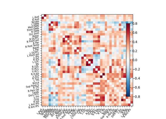
9.4.1.3. Build and display a correlation matrix

from nilearn.connectome import ConnectivityMeasure
correlation_measure = ConnectivityMeasure(kind='correlation')
correlation_matrix = correlation_measure.fit_transform([time_series])[0]

# Display the correlation matrix
import numpy as np
from nilearn import plotting
# Mask out the major diagonal
np.fill_diagonal(correlation_matrix, 0)
plotting.plot_matrix(correlation_matrix, labels=labels, colorbar=True,
                     vmax=0.8, vmin=-0.8)

Out:

/home/nicolas/GitRepos/nilearn-fork/nilearn/plotting/matrix_plotting.py:22: MatplotlibDeprecationWarning:
The inverse_transformed function was deprecated in Matplotlib 3.3 and will be removed two minor releases later. Use transformed(transform.inverted()) instead.
  ylabel_width = ax.yaxis.get_tightbbox(renderer).inverse_transformed(
/home/nicolas/GitRepos/nilearn-fork/nilearn/plotting/matrix_plotting.py:30: MatplotlibDeprecationWarning:
The inverse_transformed function was deprecated in Matplotlib 3.3 and will be removed two minor releases later. Use transformed(transform.inverted()) instead.
  xlabel_height = ax.xaxis.get_tightbbox(renderer).inverse_transformed(

<matplotlib.image.AxesImage object at 0x7f881e5b8700>

9.4.1.4. And now display the corresponding graph

from nilearn import plotting
coords = atlas.region_coords

# We threshold to keep only the 20% of edges with the highest value
# because the graph is very dense
plotting.plot_connectome(correlation_matrix, coords,
                         edge_threshold="80%", colorbar=True)

plotting.show()

9.4.1.5. 3D visualization in a web browser

An alternative to nilearn.plotting.plot_connectome is to use nilearn.plotting.view_connectome that gives more interactive visualizations in a web browser. See 3D Plots of connectomes for more details.

view = plotting.view_connectome(correlation_matrix, coords, edge_threshold='80%')

# In a Jupyter notebook, if ``view`` is the output of a cell, it will
# be displayed below the cell
view

# uncomment this to open the plot in a web browser:
# view.open_in_browser()