Note
Click here to download the full example code or to run this example in your browser via Binder
9.2.15. Making a surface plot of a 3D statistical map
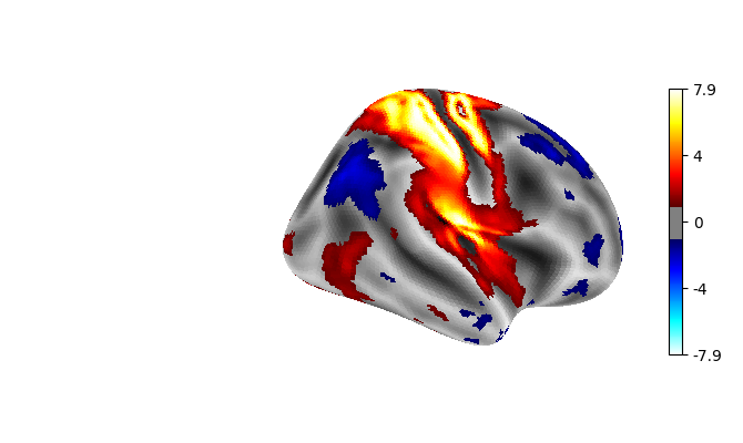
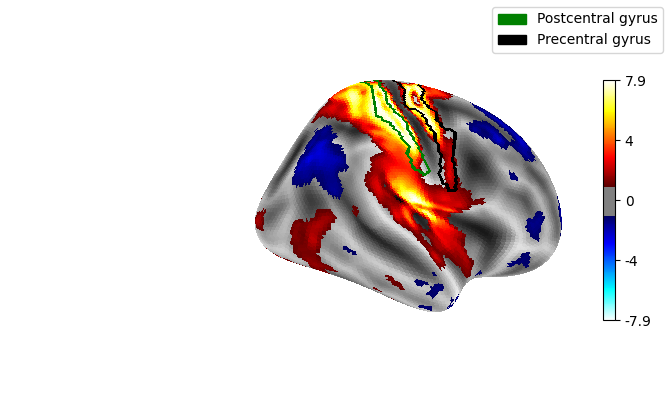
project a 3D statistical map onto a cortical mesh using nilearn.surface.vol_to_surf. Display a surface plot of the projected map using nilearn.plotting.plot_surf_stat_map and adding contours of regions of interest using nilearn.plotting.plot_surf_contours.
9.2.15.1. Get a statistical map
from nilearn import datasets
motor_images = datasets.fetch_neurovault_motor_task()
stat_img = motor_images.images[0]
9.2.15.2. Get a cortical mesh
9.2.15.3. Sample the 3D data around each node of the mesh
from nilearn import surface
texture = surface.vol_to_surf(stat_img, fsaverage.pial_right)
9.2.15.4. Plot the result
from nilearn import plotting
plotting.plot_surf_stat_map(fsaverage.infl_right, texture, hemi='right',
title='Surface right hemisphere', colorbar=True,
threshold=1., bg_map=fsaverage.sulc_right)
Out:
<Figure size 670x400 with 2 Axes>
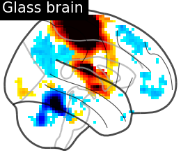
9.2.15.5. Plot 3D image for comparison
plotting.plot_glass_brain(stat_img, display_mode='r', plot_abs=False,
title='Glass brain', threshold=2.)
plotting.plot_stat_map(stat_img, display_mode='x', threshold=1.,
cut_coords=range(0, 51, 10), title='Slices')
Out:
<nilearn.plotting.displays.XSlicer object at 0x7f88203577f0>
9.2.15.6. Use an atlas and choose regions to outline
import numpy as np
destrieux_atlas = datasets.fetch_atlas_surf_destrieux()
parcellation = destrieux_atlas['map_right']
# these are the regions we want to outline
regions_dict = {b'G_postcentral': 'Postcentral gyrus',
b'G_precentral': 'Precentral gyrus'}
# get indices in atlas for these labels
regions_indices = [np.where(np.array(destrieux_atlas['labels']) == region)[0][0]
for region in regions_dict]
labels = list(regions_dict.values())
9.2.15.7. Display outlines of the regions of interest on top of a statistical map
figure = plotting.plot_surf_stat_map(fsaverage.infl_right, texture, hemi='right',
title='Surface right hemisphere',
colorbar=True, threshold=1.,
bg_map=fsaverage.sulc_right)
plotting.plot_surf_contours(fsaverage.infl_right, parcellation, labels=labels,
levels=regions_indices, figure=figure, legend=True,
colors=['g', 'k'])
plotting.show()
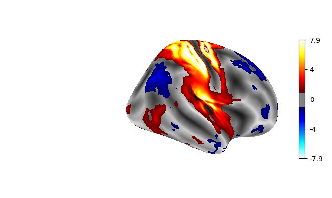
9.2.15.8. Plot with higher-resolution mesh
fetch_surf_fsaverage takes a “mesh” argument which specifies wether to fetch the low-resolution fsaverage5 mesh, or the high-resolution fsaverage mesh. using mesh=”fsaverage” will result in more memory usage and computation time, but finer visualizations.
big_fsaverage = datasets.fetch_surf_fsaverage('fsaverage')
big_texture = surface.vol_to_surf(stat_img, big_fsaverage.pial_right)
plotting.plot_surf_stat_map(big_fsaverage.infl_right,
big_texture, hemi='right', colorbar=True,
title='Surface right hemisphere: fine mesh',
threshold=1., bg_map=big_fsaverage.sulc_right)
Out:
<Figure size 670x400 with 2 Axes>
9.2.15.9. Plot multiple views of the 3D volume on a surface
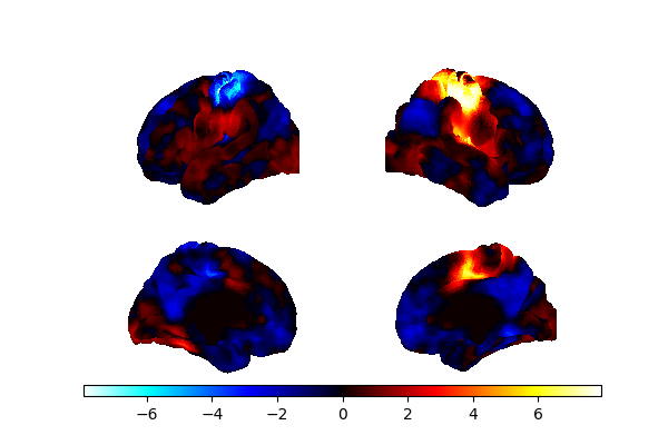
plot_img_on_surf takes a statistical map and projects it onto a surface. It supports multiple choices of orientations, and can plot either one or both hemispheres. If no surf_mesh is given, plot_img_on_surf projects the images onto FreeSurfer's fsaverage5.
plotting.plot_img_on_surf(stat_img,
views=['lateral', 'medial'],
hemispheres=['left', 'right'],
colorbar=True)
plotting.show()
9.2.15.10. 3D visualization in a web browser
An alternative to nilearn.plotting.plot_surf_stat_map is to use nilearn.plotting.view_surf or nilearn.plotting.view_img_on_surf that give more interactive visualizations in a web browser. See 3D Plots of statistical maps or atlases on the cortical surface for more details.
view = plotting.view_surf(fsaverage.infl_right, texture, threshold='90%',
bg_map=fsaverage.sulc_right)
# In a Jupyter notebook, if ``view`` is the output of a cell, it will
# be displayed below the cell
view
# uncomment this to open the plot in a web browser:
# view.open_in_browser()
We don’t need to do the projection ourselves, we can use view_img_on_surf:
view = plotting.view_img_on_surf(stat_img, threshold='90%')
# view.open_in_browser()
view
Total running time of the script: ( 0 minutes 28.876 seconds)
