NeuroImaging volumes visualization

Simple example to show Nifti data visualization.

Fetch data

from nilearn import datasets

# By default 2nd subject will be fetched
haxby_dataset = datasets.fetch_haxby()

# print basic information on the dataset
print(
    f"First anatomical nifti image (3D) located is at: {haxby_dataset.anat[0]}"
)
print(
    f"First functional nifti image (4D) is located at: {haxby_dataset.func[0]}"
)

First anatomical nifti image (3D) located is at: /home/remi/nilearn_data/haxby2001/subj2/anat.nii.gz
First functional nifti image (4D) is located at: /home/remi/nilearn_data/haxby2001/subj2/bold.nii.gz

Visualization

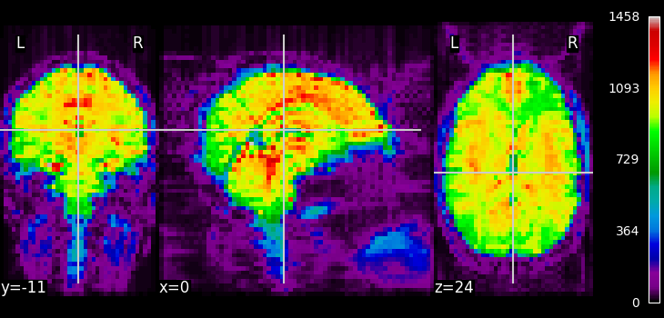
from nilearn.image.image import mean_img

# Compute the mean EPI: we do the mean along the axis 3, which is time
func_filename = haxby_dataset.func[0]
mean_haxby = mean_img(func_filename)

from nilearn.plotting import plot_epi, show

plot_epi(mean_haxby, colorbar=True, cbar_tick_format="%i")

<nilearn.plotting.displays._slicers.OrthoSlicer object at 0x7fd1f2203e10>

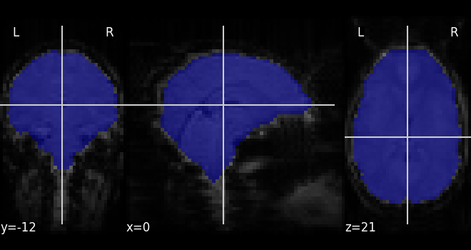
Extracting a brain mask

Simple computation of a mask from the fMRI data

from nilearn.masking import compute_epi_mask

mask_img = compute_epi_mask(func_filename)

# Visualize it as an ROI
from nilearn.plotting import plot_roi

plot_roi(mask_img, mean_haxby)

<nilearn.plotting.displays._slicers.OrthoSlicer object at 0x7fd1ed44a5d0>

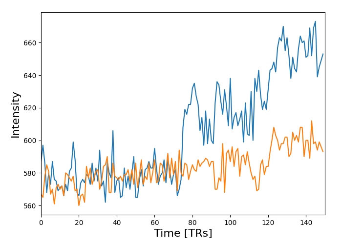
Applying the mask to extract the corresponding time series

from nilearn.masking import apply_mask

masked_data = apply_mask(func_filename, mask_img)

# masked_data shape is (timepoints, voxels). We can plot the first 150
# timepoints from two voxels

# And now plot a few of these
import matplotlib.pyplot as plt

plt.figure(figsize=(7, 5))
plt.plot(masked_data[:150, :2])
plt.xlabel("Time [TRs]", fontsize=16)
plt.ylabel("Intensity", fontsize=16)
plt.xlim(0, 150)
plt.subplots_adjust(bottom=0.12, top=0.95, right=0.95, left=0.12)

show()

Estimated memory usage: 1361 MB