Note
This page is a reference documentation. It only explains the class signature, and not how to use it. Please refer to the user guide for the big picture.
nilearn.plotting.displays.OrthoSlicer#
- class nilearn.plotting.displays.OrthoSlicer(cut_coords, axes=None, black_bg=False, brain_color=(0.5, 0.5, 0.5), **kwargs)[source]#
A class to create 3 linked axes for plotting orthogonal cuts of 3D maps. This visualization mode can be activated from Nilearn plotting functions, like
plot_img, by settingdisplay_mode='ortho':from nilearn.datasets import load_mni152_template from nilearn.plotting import plot_img img = load_mni152_template() # display is an instance of the OrthoSlicer class display = plot_img(img, display_mode='ortho')
See also
nilearn.plotting.displays.MosaicSlicerThree cuts are performed along multiple rows and columns.
nilearn.plotting.displays.TiledSlicerThree cuts are performed and arranged in a 2x2 grid.
Notes
The extent of the different axes are adjusted to fit the data best in the viewing area.
- Attributes
- classmethod find_cut_coords(img=None, threshold=None, cut_coords=None)[source]#
Instantiate the slicer and find cut coordinates.
- Parameters
- %(img)s
- threshold
intorfloatorNone, optional Threshold to apply:
If
Noneis given, the maps are not thresholded.If a number is given, it is used to threshold the maps, values below the threshold (in absolute value) are plotted as transparent.
Default=None.
- cut_coords3
tupleofint The cut position, in world space.
- draw_cross(cut_coords=None, **kwargs)[source]#
Draw a crossbar on the plot to show where the cut is performed.
- add_contours(img, threshold=1e-06, filled=False, **kwargs)[source]#
Contour a 3D map in all the views.
- Parameters
- imgNiimg-like object
See Input and output: neuroimaging data representation. Provides image to plot.
- threshold
intorfloatorNone, optional Threshold to apply:
If
Noneis given, the maps are not thresholded.If a number is given, it is used to threshold the maps, values below the threshold (in absolute value) are plotted as transparent.
Default=1e-6.
- filled
bool, optional If
filled=True, contours are displayed with color fillings. Default=False.- kwargs
dict Extra keyword arguments are passed to function
contour, or functioncontourf. Useful, arguments are typical “levels”, which is a list of values to use for plotting a contour or contour fillings (iffilled=True), and “colors”, which is one color or a list of colors for these contours.
Notes
If colors are not specified, default coloring choices (from matplotlib) for contours and contour_fillings can be different.
- add_edges(img, color='r')[source]#
Plot the edges of a 3D map in all the views.
- Parameters
- imgNiimg-like object
See Input and output: neuroimaging data representation. The 3D map to be plotted. If it is a masked array, only the non-masked part will be plotted.
- colormatplotlib color:
stror (r, g, b) value The color used to display the edge map. Default=’r’.
- add_markers(marker_coords, marker_color='r', marker_size=30, **kwargs)[source]#
Add markers to the plot.
- Parameters
- marker_coords
ndarrayof shape(n_markers, 3) Coordinates of the markers to plot. For each slice, only markers that are 2 millimeters away from the slice are plotted.
- marker_colorpyplot compatible color or
listof shape(n_markers,), optional List of colors for each marker that can be string or matplotlib colors. Default=’r’.
- marker_size
floatorlistoffloatof shape(n_markers,), optional Size in pixel for each marker. Default=30.
- marker_coords
- add_overlay(img, threshold=1e-06, colorbar=False, cbar_tick_format='%.2g', cbar_vmin=None, cbar_vmax=None, **kwargs)[source]#
Plot a 3D map in all the views.
- Parameters
- imgNiimg-like object
See Input and output: neuroimaging data representation. If it is a masked array, only the non-masked part will be plotted.
- threshold
intorfloatorNone, optional Threshold to apply:
If
Noneis given, the maps are not thresholded.If a number is given, it is used to threshold the maps: values below the threshold (in absolute value) are plotted as transparent.
Default=1e-6.
- cbar_tick_format: str, optional
Controls how to format the tick labels of the colorbar. Ex: use “%i” to display as integers. Default is ‘%.2g’ for scientific notation.
- colorbar
bool, optional If
True, display a colorbar on the right of the plots. Default=False.- kwargs
dict Extra keyword arguments are passed to function
imshow.- cbar_vmin
float, optional Minimal value for the colorbar. If None, the minimal value is computed based on the data.
- cbar_vmax
float, optional Maximal value for the colorbar. If None, the maximal value is computed based on the data.
- annotate(left_right=True, positions=True, scalebar=False, size=12, scale_size=5.0, scale_units='cm', scale_loc=4, decimals=0, **kwargs)[source]#
Add annotations to the plot.
- Parameters
- left_right
bool, optional If
True, annotations indicating which side is left and which side is right are drawn. Default=True.- positions
bool, optional If
True, annotations indicating the positions of the cuts are drawn. Default=True.- scalebar
bool, optional If
True, cuts are annotated with a reference scale bar. For finer control of the scale bar, please check out thedraw_scale_barmethod on the axes in “axes” attribute of this object. Default=False.- size
int, optional The size of the text used. Default=12.
- scale_size
intorfloat, optional The length of the scalebar, in units of
scale_units. Default=5.0.- scale_units{‘cm’, ‘mm’}, optional
The units for the
scalebar. Default=’cm’.- scale_loc
int, optional The positioning for the scalebar. Default=4. Valid location codes are:
1: “upper right”
2: “upper left”
3: “lower left”
4: “lower right”
5: “right”
6: “center left”
7: “center right”
8: “lower center”
9: “upper center”
10: “center”
- decimals
int, optional Number of decimal places on slice position annotation. If zero, the slice position is integer without decimal point. Default=0.
- kwargs
dict Extra keyword arguments are passed to matplotlib’s text function.
- left_right
- property black_bg#
- property brain_color#
- classmethod init_with_figure(img, threshold=None, cut_coords=None, figure=None, axes=None, black_bg=False, leave_space=False, colorbar=False, brain_color=(0.5, 0.5, 0.5), **kwargs)[source]#
Initialize the slicer with an image.
- Parameters
- imgNiimg-like object
- cut_coords3
tupleofint The cut position, in world space.
- axes
matplotlib.axes.Axes, optional The axes that will be subdivided in 3.
- black_bg
bool, optional If
True, the background of the figure will be put to black. If you wish to save figures with a black background, you will need to passfacecolor='k', edgecolor='k'tomatplotlib.pyplot.savefig. Default=False.- brain_color
tuple, optional The brain color to use as the background color (e.g., for transparent colorbars). Default=(0.5, 0.5, 0.5).
- savefig(filename, dpi=None)[source]#
Save the figure to a file.
- Parameters
- filename
str The file name to save to. Its extension determines the file type, typically ‘.png’, ‘.svg’ or ‘.pdf’.
- dpi
Noneor scalar, optional The resolution in dots per inch. Default=None.
- filename
- title(text, x=0.01, y=0.99, size=15, color=None, bgcolor=None, alpha=1, **kwargs)[source]#
Write a title to the view.
- Parameters
- text
str The text of the title.
- x
float, optional The horizontal position of the title on the frame in fraction of the frame width. Default=0.01.
- y
float, optional The vertical position of the title on the frame in fraction of the frame height. Default=0.99.
- size
int, optional The size of the title text. Default=15.
- colormatplotlib color specifier, optional
The color of the font of the title.
- bgcolormatplotlib color specifier, optional
The color of the background of the title.
- alpha
float, optional The alpha value for the background. Default=1.
- kwargs
Extra keyword arguments are passed to matplotlib’s text function.
- text
Examples using nilearn.plotting.displays.OrthoSlicer#
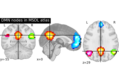
Visualizing a probabilistic atlas: the default mode in the MSDL atlas
Producing single subject maps of seed-to-voxel correlation
Regions extraction using dictionary learning and functional connectomes
Beta-Series Modeling for Task-Based Functional Connectivity and Decoding
