Note
Click here to download the full example code or to run this example in your browser via Binder
Functional connectivity predicts age group#
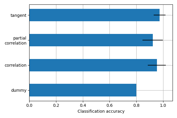
This example compares different kinds of functional connectivity between regions of interest : correlation, partial correlation, and tangent space embedding.
The resulting connectivity coefficients can be used to discriminate children from adults. In general, the tangent space embedding outperforms the standard correlations: see Dadi et al 2019 for a careful study.
Note
If you are using Nilearn with a version older than 0.9.0, then you should either upgrade your version or import maskers from the input_data module instead of the maskers module.
That is, you should manually replace in the following example all occurrences of:
from nilearn.maskers import NiftiMasker
with:
from nilearn.input_data import NiftiMasker
Load brain development fMRI dataset and MSDL atlas#
We study only 60 subjects from the dataset, to save computation time.
from nilearn import datasets

development_dataset = datasets.fetch_development_fmri(n_subjects=60)
We use probabilistic regions of interest (ROIs) from the MSDL atlas.
from nilearn.maskers import NiftiMapsMasker

msdl_data = datasets.fetch_atlas_msdl()
msdl_coords = msdl_data.region_coords

masker = NiftiMapsMasker(
    msdl_data.maps, resampling_target="data", t_r=2, detrend=True,
    low_pass=.1, high_pass=.01, memory='nilearn_cache', memory_level=1).fit()
masked_data = [masker.transform(func, confounds) for
               (func, confounds) in zip(
                   development_dataset.func, development_dataset.confounds)]
What kind of connectivity is most powerful for classification?#
we will use connectivity matrices as features to distinguish children from adults. We use cross-validation and measure classification accuracy to compare the different kinds of connectivity matrices.
# prepare the classification pipeline
from sklearn.pipeline import Pipeline
from nilearn.connectome import ConnectivityMeasure
from sklearn.svm import LinearSVC
from sklearn.dummy import DummyClassifier
from sklearn.model_selection import GridSearchCV

kinds = ['correlation', 'partial correlation', 'tangent']

pipe = Pipeline(
    [('connectivity', ConnectivityMeasure(vectorize=True)),
     ('classifier', GridSearchCV(LinearSVC(), {'C': [.1, 1., 10.]}, cv=5))])

param_grid = [
    {'classifier': [DummyClassifier(strategy='most_frequent')]},
    {'connectivity__kind': kinds}
]
We use random splits of the subjects into training/testing sets. StratifiedShuffleSplit allows preserving the proportion of children in the test set.
from sklearn.model_selection import GridSearchCV, StratifiedShuffleSplit
from sklearn.preprocessing import LabelEncoder

groups = [pheno['Child_Adult'] for pheno in development_dataset.phenotypic]
classes = LabelEncoder().fit_transform(groups)

cv = StratifiedShuffleSplit(n_splits=30, random_state=0, test_size=10)
gs = GridSearchCV(pipe, param_grid, scoring='accuracy', cv=cv, verbose=1,
                  refit=False, n_jobs=8)
gs.fit(masked_data, classes)
mean_scores = gs.cv_results_['mean_test_score']
scores_std = gs.cv_results_['std_test_score']
Fitting 30 folds for each of 4 candidates, totalling 120 fits
display the results
from matplotlib import pyplot as plt

plt.figure(figsize=(6, 4))
positions = [.1, .2, .3, .4]
plt.barh(positions, mean_scores, align='center', height=.05, xerr=scores_std)
yticks = ['dummy'] + list(gs.cv_results_['param_connectivity__kind'].data[1:])
yticks = [t.replace(' ', '\n') for t in yticks]
plt.yticks(positions, yticks)
plt.xlabel('Classification accuracy')
plt.gca().grid(True)
plt.gca().set_axisbelow(True)
plt.tight_layout()

This is a small example to showcase nilearn features. In practice such comparisons need to be performed on much larger cohorts and several datasets. Dadi et al 2019 Showed that across many cohorts and clinical questions, the tangent kind should be preferred.
plt.show()
Total running time of the script: ( 2 minutes 1.943 seconds)
Estimated memory usage: 1187 MB