Example of explicit fixed effects fMRI model fitting

This example illustrates how to run a fixed effects model based on pre-computed statistics. This is helpful when the initial models have to be fit separately.

For details on the data, please see:

Dehaene-Lambertz G, Dehaene S, Anton JL, Campagne A, Ciuciu P, Dehaene

G, Denghien I, Jobert A, LeBihan D, Sigman M, Pallier C, Poline JB. Functional segregation of cortical language areas by sentence repetition. Hum Brain Mapp. 2006: 27:360–371. http://www.pubmedcentral.nih.gov/articlerender.fcgi?artid=2653076#R11

Please see Simple example of two-session fMRI model fitting for details. The main difference is that the fixed-effects model is run explicitly here, after GLM fitting on two sessions.

Prepare data and analysis parameters

Inspecting ‘data’, we note that there are two sessions

from nilearn.datasets import func
data = func.fetch_fiac_first_level()
fmri_img = [data['func1'], data['func2']]

Create a mean image for plotting purpose

from nilearn.image import mean_img
mean_img_ = mean_img(fmri_img[0])

The design matrices were pre-computed, we simply put them in a list of DataFrames

design_files = [data['design_matrix1'], data['design_matrix2']]
import pandas as pd
import numpy as np
design_matrices = [pd.DataFrame(np.load(df)['X']) for df in design_files]

GLM estimation

GLM specification. Note that the mask was provided in the dataset. So we use it.

from nilearn.glm.first_level import FirstLevelModel
fmri_glm = FirstLevelModel(mask_img=data['mask'], smoothing_fwhm=5,
                           minimize_memory=True)

Compute fixed effects of the two runs and compute related images For this, we first define the contrasts as we would do for a single session

n_columns = design_matrices[0].shape[1]
contrast_val = np.hstack(([-1, -1, 1, 1], np.zeros(n_columns - 4)))

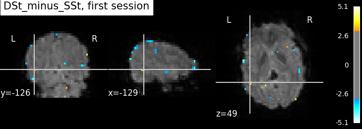
Statistics for the first session

from nilearn import plotting
cut_coords = [-129, -126, 49]
contrast_id = 'DSt_minus_SSt'

fmri_glm = fmri_glm.fit(fmri_img[0], design_matrices=design_matrices[0])
summary_statistics_session1 = fmri_glm.compute_contrast(
    contrast_val, output_type='all')
plotting.plot_stat_map(
    summary_statistics_session1['z_score'],
    bg_img=mean_img_, threshold=3.0, cut_coords=cut_coords,
    title='{0}, first session'.format(contrast_id))

<nilearn.plotting.displays._slicers.OrthoSlicer object at 0x7fc1a8ee0b50>

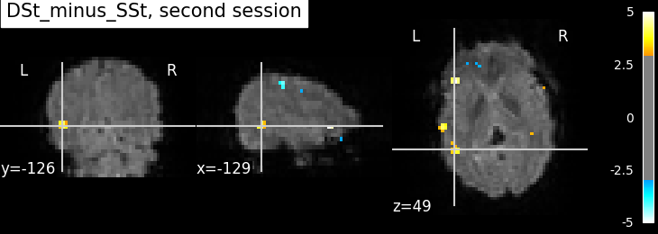
Statistics for the second session

fmri_glm = fmri_glm.fit(fmri_img[1], design_matrices=design_matrices[1])
summary_statistics_session2 = fmri_glm.compute_contrast(
    contrast_val, output_type='all')
plotting.plot_stat_map(
    summary_statistics_session2['z_score'],
    bg_img=mean_img_, threshold=3.0, cut_coords=cut_coords,
    title='{0}, second session'.format(contrast_id))

<nilearn.plotting.displays._slicers.OrthoSlicer object at 0x7fc1a5d38df0>

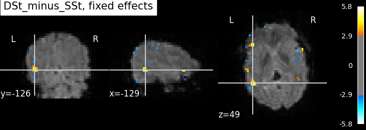
Fixed effects statistics

from nilearn.glm.contrasts import compute_fixed_effects

contrast_imgs = [summary_statistics_session1['effect_size'],
                 summary_statistics_session2['effect_size']]
variance_imgs = [summary_statistics_session1['effect_variance'],
                 summary_statistics_session2['effect_variance']]

fixed_fx_contrast, fixed_fx_variance, fixed_fx_stat = compute_fixed_effects(
    contrast_imgs, variance_imgs, data['mask'])
plotting.plot_stat_map(
    fixed_fx_stat, bg_img=mean_img_, threshold=3.0, cut_coords=cut_coords,
    title='{0}, fixed effects'.format(contrast_id))

<nilearn.plotting.displays._slicers.OrthoSlicer object at 0x7fc1a8ee27a0>

Not unexpectedly, the fixed effects version displays higher peaks than the input sessions. Computing fixed effects enhances the signal-to-noise ratio of the resulting brain maps Note however that, technically, the output maps of the fixed effects map is a t statistic (not a z statistic)

plotting.show()

Estimated memory usage: 481 MB