Note
Click here to download the full example code or to run this example in your browser via Binder
Extract signals on spheres and plot a connectome#
This example shows how to extract signals from spherical regions. We show how to build spheres around user-defined coordinates, as well as centered on coordinates from the Power-264 atlas [1], and the Dosenbach-160 atlas [2].
Note
If you are using Nilearn with a version older than 0.9.0, then you should either upgrade your version or import maskers from the input_data module instead of the maskers module.
That is, you should manually replace in the following example all occurrences of:
from nilearn.maskers import NiftiMasker
with:
from nilearn.input_data import NiftiMasker
References
[1] Power, Jonathan D., et al. “Functional network organization of the human brain.” Neuron 72.4 (2011): 665-678.
[2] Dosenbach N.U., Nardos B., et al. “Prediction of individual brain maturity using fMRI.”, 2010, Science 329, 1358-1361.
We estimate connectomes using two different methods: sparse inverse covariance and partial_correlation, to recover the functional brain networks structure.
We’ll start by extracting signals from Default Mode Network regions and computing a connectome from them.
Retrieve the brain development fmri dataset#
We are going to use a subject from the development functional connectivity dataset.
from nilearn import datasets
dataset = datasets.fetch_development_fmri(n_subjects=10)

# print basic information on the dataset
print('First subject functional nifti image (4D) is at: %s' %
      dataset.func[0])  # 4D data
First subject functional nifti image (4D) is at: /home/yasmin/nilearn/nilearn_data/development_fmri/development_fmri/sub-pixar123_task-pixar_space-MNI152NLin2009cAsym_desc-preproc_bold.nii.gz
Coordinates of Default Mode Network#
dmn_coords = [(0, -52, 18), (-46, -68, 32), (46, -68, 32), (1, 50, -5)]
labels = [
    'Posterior Cingulate Cortex',
    'Left Temporoparietal junction',
    'Right Temporoparietal junction',
    'Medial prefrontal cortex',
]
Extracts signal from sphere around DMN seeds#
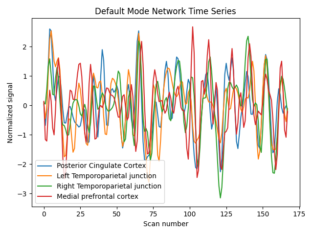
We can compute the mean signal within spheres of a fixed radius around a sequence of (x, y, z) coordinates with the object nilearn.maskers.NiftiSpheresMasker. The resulting signal is then prepared by the masker object: Detrended, band-pass filtered and standardized to 1 variance.
from nilearn.maskers import NiftiSpheresMasker

masker = NiftiSpheresMasker(
    dmn_coords, radius=8, detrend=True, standardize=True,
    low_pass=0.1, high_pass=0.01, t_r=2,
    memory='nilearn_cache', memory_level=1, verbose=2)

# Additionally, we pass confound information to ensure our extracted
# signal is cleaned from confounds.

func_filename = dataset.func[0]
confounds_filename = dataset.confounds[0]

time_series = masker.fit_transform(func_filename,
                                   confounds=[confounds_filename])
________________________________________________________________________________
[Memory] Calling nilearn.maskers.base_masker._filter_and_extract...
_filter_and_extract('/home/yasmin/nilearn/nilearn_data/development_fmri/development_fmri/sub-pixar123_task-pixar_space-MNI152NLin2009cAsym_desc-preproc_bold.nii.gz',
<nilearn.maskers.nifti_spheres_masker._ExtractionFunctor object at 0x7fc1ef1d8580>,
{ 'allow_overlap': False,
  'detrend': True,
  'dtype': None,
  'high_pass': 0.01,
  'high_variance_confounds': False,
  'low_pass': 0.1,
  'mask_img': None,
  'radius': 8,
  'seeds': [(0, -52, 18), (-46, -68, 32), (46, -68, 32), (1, 50, -5)],
  'smoothing_fwhm': None,
  'standardize': True,
  'standardize_confounds': True,
  't_r': 2}, confounds=[ '/home/yasmin/nilearn/nilearn_data/development_fmri/development_fmri/sub-pixar123_task-pixar_desc-reducedConfounds_regressors.tsv'], sample_mask=None, dtype=None, memory=Memory(location=nilearn_cache/joblib), memory_level=1, verbose=2)
[NiftiSpheresMasker.transform_single_imgs] Loading data from /home/yasmin/nilearn/nilearn_data/development_fmri/development_fmri/sub-pixar123_task-pixar_space-MNI152NLin2009cAsym_desc-preproc_bold.nii.gz
[NiftiSpheresMasker.transform_single_imgs] Extracting region signals
[NiftiSpheresMasker.transform_single_imgs] Cleaning extracted signals
_______________________________________________filter_and_extract - 2.4s, 0.0min
Display time series#
import matplotlib.pyplot as plt

for time_serie, label in zip(time_series.T, labels):
    plt.plot(time_serie, label=label)

plt.title('Default Mode Network Time Series')
plt.xlabel('Scan number')
plt.ylabel('Normalized signal')
plt.legend()
plt.tight_layout()
Compute partial correlation matrix#
Using object nilearn.connectome.ConnectivityMeasure: Its default covariance estimator is Ledoit-Wolf, allowing to obtain accurate partial correlations.
from nilearn.connectome import ConnectivityMeasure
connectivity_measure = ConnectivityMeasure(kind='partial correlation')
partial_correlation_matrix = connectivity_measure.fit_transform(
    [time_series])[0]
Display connectome#
We display the graph of connections with :func: nilearn.plotting.plot_connectome.
from nilearn import plotting

plotting.plot_connectome(partial_correlation_matrix, dmn_coords,
                         title="Default Mode Network Connectivity")
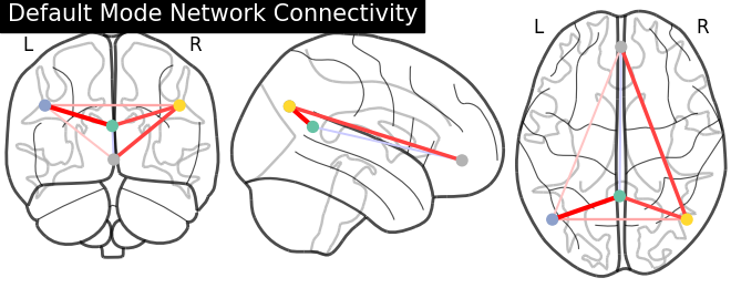
<nilearn.plotting.displays._projectors.OrthoProjector object at 0x7fc1aac40070>
Display connectome with hemispheric projections. Notice (0, -52, 18) is included in both hemispheres since x == 0.
plotting.plot_connectome(partial_correlation_matrix, dmn_coords,
                         title="Connectivity projected on hemispheres",
                         display_mode='lyrz')

plotting.show()

3D visualization in a web browser#
An alternative to nilearn.plotting.plot_connectome is to use nilearn.plotting.view_connectome, which gives more interactive visualizations in a web browser. See 3D Plots of connectomes for more details.
view = plotting.view_connectome(partial_correlation_matrix, dmn_coords)

# In a Jupyter notebook, if ``view`` is the output of a cell, it will
# be displayed below the cell
view
# uncomment this to open the plot in a web browser:
# view.open_in_browser()
Extract signals on spheres from an atlas#
Next, instead of supplying our own coordinates, we will use coordinates generated at the center of mass of regions from two different atlases. This time, we’ll use a different correlation measure.
First we fetch the coordinates of the Power atlas
power = datasets.fetch_coords_power_2011(legacy_format=False)
print('Power atlas comes with {0}.'.format(power.keys()))
Power atlas comes with dict_keys(['rois', 'description']).
Note
You can retrieve the coordinates for any atlas, including atlases not included in nilearn, using nilearn.plotting.find_parcellation_cut_coords.
Compute within spheres averaged time-series#
We collect the regions coordinates in a numpy array
import numpy as np

coords = np.vstack((power.rois['x'], power.rois['y'], power.rois['z'])).T

print('Stacked power coordinates in array of shape {0}.'.format(coords.shape))
Stacked power coordinates in array of shape (264, 3).
and define spheres masker, with small enough radius to avoid regions overlap.
spheres_masker = NiftiSpheresMasker(
    seeds=coords, smoothing_fwhm=6, radius=5.,
    detrend=True, standardize=True, low_pass=0.1, high_pass=0.01, t_r=2)

timeseries = spheres_masker.fit_transform(func_filename,
                                          confounds=confounds_filename)
Estimate correlations#
We start by estimating the signal covariance matrix. Here the number of ROIs exceeds the number of samples,
print('time series has {0} samples'.format(timeseries.shape[0]))
time series has 168 samples
in which situation the graphical lasso sparse inverse covariance estimator captures well the covariance structure.
try:
    from sklearn.covariance import GraphicalLassoCV
except ImportError:
    # for Scitkit-Learn < v0.20.0
    from sklearn.covariance import GraphLassoCV as GraphicalLassoCV

covariance_estimator = GraphicalLassoCV(cv=3, verbose=1)
We just fit our regions signals into the GraphicalLassoCV object
[Parallel(n_jobs=1)]: Using backend SequentialBackend with 1 concurrent workers.
[Parallel(n_jobs=1)]: Done   3 out of   3 | elapsed:   23.6s finished
[GraphicalLassoCV] Done refinement  1 out of 4:  23s
[Parallel(n_jobs=1)]: Using backend SequentialBackend with 1 concurrent workers.
[Parallel(n_jobs=1)]: Done   3 out of   3 | elapsed:   50.6s finished
[GraphicalLassoCV] Done refinement  2 out of 4:  74s
[Parallel(n_jobs=1)]: Using backend SequentialBackend with 1 concurrent workers.
[Parallel(n_jobs=1)]: Done   3 out of   3 | elapsed:   53.5s finished
[GraphicalLassoCV] Done refinement  3 out of 4:  127s
[Parallel(n_jobs=1)]: Using backend SequentialBackend with 1 concurrent workers.
[Parallel(n_jobs=1)]: Done   3 out of   3 | elapsed:   52.9s finished
[GraphicalLassoCV] Done refinement  4 out of 4:  180s
/home/yasmin/miniconda3/envs/nilearn-dev/lib/python3.10/site-packages/numpy/core/_methods.py:233: RuntimeWarning:

invalid value encountered in subtract
and get the ROI-to-ROI covariance matrix.
matrix = covariance_estimator.covariance_
print('Covariance matrix has shape {0}.'.format(matrix.shape))
Covariance matrix has shape (264, 264).
Plot matrix, graph, and strength#
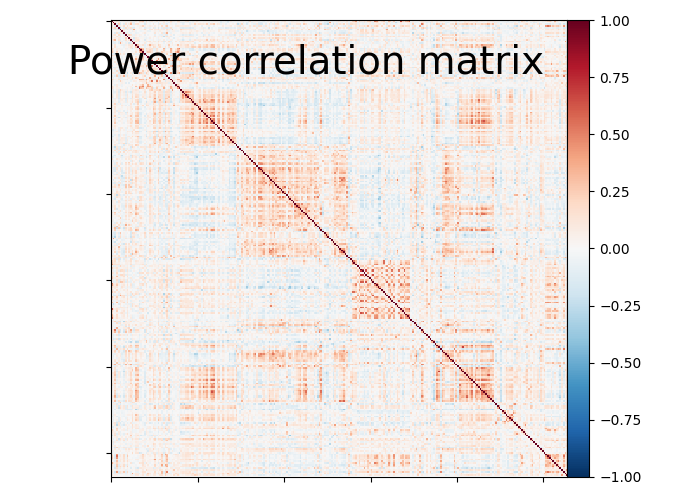
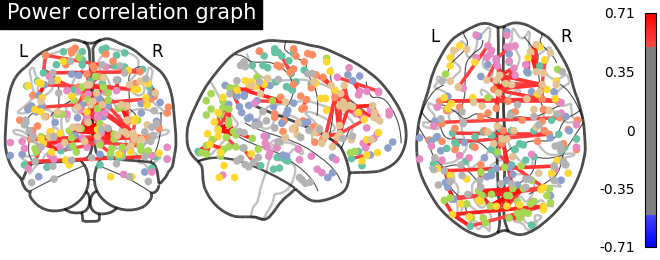
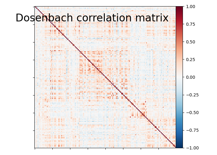
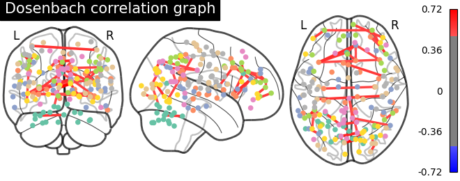
We use :func: nilearn.plotting.plot_matrix to visualize our correlation matrix and display the graph of connections with nilearn.plotting.plot_connectome.
from nilearn import plotting

plotting.plot_matrix(matrix, vmin=-1., vmax=1., colorbar=True,
                     title='Power correlation matrix')

# Tweak edge_threshold to keep only the strongest connections.
plotting.plot_connectome(matrix, coords, title='Power correlation graph',
                         edge_threshold='99.8%', node_size=20, colorbar=True)
<nilearn.plotting.displays._projectors.OrthoProjector object at 0x7fc1ab83b7c0>
Note
Note the 1. on the matrix diagonal: These are the signals variances, set to 1. by the spheres_masker. Hence the covariance of the signal is a correlation matrix.
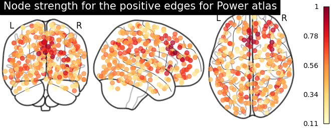
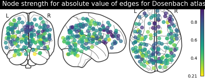
Sometimes, the information in the correlation matrix is overwhelming and aggregating edge strength from the graph would help. Use the function nilearn.plotting.plot_markers to visualize this information.
# calculate normalized, absolute strength for each node
node_strength = np.sum(np.abs(matrix), axis=0)
node_strength /= np.max(node_strength)

plotting.plot_markers(
    node_strength,
    coords,
    title='Node strength for absolute value of edges for Power atlas',
)
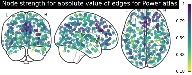
<nilearn.plotting.displays._projectors.OrthoProjector object at 0x7fc1a8046230>
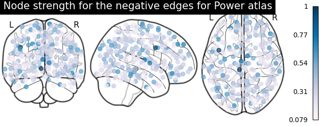
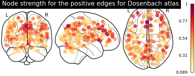
From the correlation matrix, we observe that there is a positive and negative structure. We could make two different plots, one for the positive and one for the negative structure.
from matplotlib.pyplot import cm

# clip connectivity matrix to preserve positive and negative edges
positive_edges = np.clip(matrix, 0, matrix.max())
negative_edges = np.clip(matrix, matrix.min(), 0)

# calculate strength for positive edges
node_strength_positive = np.sum(np.abs(positive_edges), axis=0)
node_strength_positive /= np.max(node_strength_positive)

# calculate strength for negative edges
node_strength_negative = np.sum(np.abs(negative_edges), axis=0)
node_strength_negative /= np.max(node_strength_negative)

# plot nodes' strength for positive edges
plotting.plot_markers(
    node_strength_positive,
    coords,
    title='Node strength for the positive edges for Power atlas',
    node_cmap=cm.YlOrRd
)

# plot nodes' strength for negative edges
plotting.plot_markers(
    node_strength_negative,
    coords,
    title='Node strength for the negative edges for Power atlas',
    node_cmap=cm.PuBu
)
<nilearn.plotting.displays._projectors.OrthoProjector object at 0x7fc1a8f34d60>
Connectome extracted from Dosenbach’s atlas#
We repeat the same steps for Dosenbach’s atlas.
dosenbach = datasets.fetch_coords_dosenbach_2010(legacy_format=False)

coords = np.vstack((
    dosenbach.rois['x'],
    dosenbach.rois['y'],
    dosenbach.rois['z'],
)).T

spheres_masker = NiftiSpheresMasker(
    seeds=coords, smoothing_fwhm=6, radius=4.5,
    detrend=True, standardize=True, low_pass=0.1, high_pass=0.01, t_r=2)

timeseries = spheres_masker.fit_transform(func_filename,
                                          confounds=confounds_filename)

covariance_estimator = GraphicalLassoCV()
covariance_estimator.fit(timeseries)
matrix = covariance_estimator.covariance_

plotting.plot_matrix(matrix, vmin=-1., vmax=1., colorbar=True,
                     title='Dosenbach correlation matrix')

plotting.plot_connectome(matrix, coords, title='Dosenbach correlation graph',
                         edge_threshold="99.7%", node_size=20, colorbar=True)


# calculate average strength for each node
node_strength = np.sum(np.abs(matrix), axis=0)
node_strength /= np.max(node_strength)

plotting.plot_markers(
    node_strength,
    coords,
    title='Node strength for absolute value of edges for Dosenbach atlas',
)

# clip connectivity matrix to preserve positive and negative edges
positive_edges = np.clip(matrix, 0, matrix.max())
negative_edges = np.clip(matrix, matrix.min(), 0)

# calculate strength for positive and edges
node_strength_positive = np.sum(np.abs(positive_edges), axis=0)
node_strength_positive /= np.max(node_strength_positive)
node_strength_negative = np.sum(np.abs(negative_edges), axis=0)
node_strength_negative /= np.max(node_strength_negative)

# plot nodes' strength for positive edges
plotting.plot_markers(
    node_strength_positive,
    coords,
    title='Node strength for the positive edges for Dosenbach atlas',
    node_cmap=cm.YlOrRd
)

# plot nodes' strength for negative edges
plotting.plot_markers(
    node_strength_negative,
    coords,
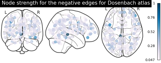
    title='Node strength for the negative edges for Dosenbach atlas',
    node_cmap=cm.PuBu
)
/home/yasmin/miniconda3/envs/nilearn-dev/lib/python3.10/site-packages/numpy/core/_methods.py:233: RuntimeWarning:

invalid value encountered in subtract


<nilearn.plotting.displays._projectors.OrthoProjector object at 0x7fc1a5a6a020>
We can easily identify the Dosenbach’s networks from the matrix blocks.
print('Dosenbach networks names are {0}'.format(np.unique(dosenbach.networks)))

plotting.show()
Dosenbach networks names are ['cerebellum' 'cingulo-opercular' 'default' 'fronto-parietal' 'occipital'
 'sensorimotor']
References#
See also#
Total running time of the script: ( 5 minutes 47.491 seconds)
Estimated memory usage: 577 MB
